Back to the on-screen lesson ·
Split total variation into explained and residual sums of squares, compute R-squared, and say what it does not measure.
Paper packet. Every task here also exists on screen, where it is checked automatically; answers written on paper are not assessed by Nydus. When you are back at a device, enter your answers there.
By the end of this lesson you will be able to compute fitted values, residuals and the sums of squares, find R-squared two ways, and judge what a given R-squared does and does not show.
From the last lesson you can fit an OLS line by hand and you know its residuals sum to zero and are uncorrelated with $x$. From statistics you know the variance as an average squared deviation from the mean.
This lesson asks how well the line fits. It splits the total variation in $y$ into the part the line explains and the part it leaves in the residuals, and turns the split into one number, $R^2$ — then explains why that number answers much less than people expect.
| Term | What it means |
|---|---|
| Fitted value | $\hat y_i = \hat\beta_0 + \hat\beta_1 x_i$, the point on the line above $x_i$. |
| Residual | $\hat u_i = y_i - \hat y_i$, the vertical gap from the point to the line. |
| SST | Total sum of squares, $\sum (y_i - \bar y)^2$: all the variation in $y$. |
| SSE | Explained sum of squares, $\sum (\hat y_i - \bar y)^2$: variation in the fitted values. |
| SSR | Sum of squared residuals, $\sum \hat u_i^2$: variation the line leaves over. |
| R-squared | $R^2 = SSE/SST = 1 - SSR/SST$, the share of sample variation in $y$ explained. |
| Goodness of fit | How closely the data points lie to the fitted line. |
Every observation can be split into a fitted part and a residual: $y_i = \hat y_i + \hat u_i$. Subtract $\bar y$ from both sides and square. Because OLS residuals are uncorrelated with the fitted values, the cross term sums to zero, and the squares add up cleanly:
$$\underbrace{\sum (y_i - \bar y)^2}_{SST} = \underbrace{\sum (\hat y_i - \bar y)^2}_{SSE} + \underbrace{\sum \hat u_i^2}_{SSR}.$$
The share explained is $R^2 = SSE/SST = 1 - SSR/SST$. It is $0$ when the line is flat and explains nothing, $1$ when every point sits on the line, and in between otherwise. With one regressor it equals the squared correlation of $x$ and $y$.
Textbooks disagree about the letters: some call the explained sum SSR, for regression, and the residual sum SSE, for error. The meaning is what matters: always check which one is left over.
Another way: action
On a scatterplot, draw the horizontal line at $\bar y$ and the fitted line. For one point, mark the vertical distance to the mean (total), from the mean to the line (explained) and from the line to the point (residual).
Another way: steps
Write $y_i - \bar y = (\hat y_i - \bar y) + \hat u_i$ and square it. You get the two squares plus twice the cross product $\sum (\hat y_i - \bar y)\hat u_i$.
That cross product is zero because of the normal equations from the last lesson. The residuals sum to zero, which kills the $\bar y$ part, and the residuals are uncorrelated with $x$, so they are uncorrelated with any linear function of $x$, including the fitted values. So OLS splits the variation into two pieces that do not overlap.
This is special to least squares with an intercept. Fit a line some other way, or force it through the origin, and the pieces no longer add up; $R^2$ computed the two ways can even disagree.
$R^2$ answers one question: how closely do these sample points cluster around this line? It is silent on the questions a policy analyst usually cares about.
In cross-section data on people, $R^2$ of $0.1$ to $0.3$ is normal and says only that individuals differ in many ways the regression does not measure. In time series of trending variables, $R^2$ near $1$ is common and often meaningless.
Residuals and the three sums of squares are in the units of $y$ (squared, for the sums). $R^2$ has no units: it is a ratio of two sums of squares measured the same way.
That makes it convenient for comparing fits of the same $y$ with different regressors, but dangerous for comparing across different outcome variables. A regression of log wages and a regression of wages can have very different $R^2$ with the same information, because the total variation being explained is different. Compare $R^2$ only between models of the same dependent variable, estimated on the same sample.
Residuals, by contrast, keep the units of the outcome and are worth reading one by one. A residual of $-3$ in a sales regression says that week sold three thousand units fewer than weeks with the same advertising did on average. Sorting observations by their residuals is a quick way to find data errors, unusual cases and patterns the line has missed, such as every holiday week sitting well above it. A pattern in the residuals is a hint that the model needs another variable or a different shape, and it is often the first clue an analyst gets.
In the next unit, regressions get more than one explanatory variable. One warning belongs here, because it is about fit. Adding any variable to a regression, even a column of random numbers, can never lower $R^2$ and almost always raises it a little. The reason is mechanical: with an extra coefficient to choose, least squares can do at least as well as before by setting it to zero, and usually finds some small value that shaves a bit off the residuals by chance.
So a higher $R^2$ from a bigger model is not evidence that the new variable matters. The adjusted $R^2$ charges a penalty for each extra coefficient, and can fall when a useless variable is added. Better still, later lessons test whether new variables matter with an F-test, which asks whether the improvement in fit is larger than chance alone would produce.
The deeper lesson is that fit is cheap. With enough variables, any dataset can be fitted closely. What is expensive, and what an econometrician is paid for, is a credible argument that a particular coefficient answers a particular question.
When the goal is prediction, fit is exactly the right target, but it must be measured on data the model has not seen. A model that fits its own sample with $R^2 = 0.95$ can predict new cases badly if it has chased noise. Forecasters therefore hold back part of the data, fit on the rest, and judge the model by how well it predicts the held-back part.
When the goal is a causal effect, fit is almost beside the point. The question is whether the variation in $x$ used to estimate the slope is free of selection. A randomized experiment with $R^2 = 0.02$ can give a far more trustworthy effect than an observational regression with $R^2 = 0.8$.
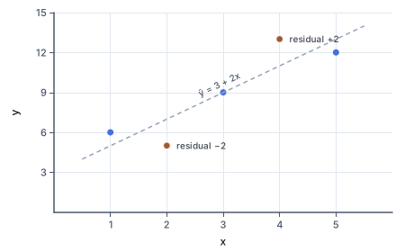
The figure plots these five points and the fitted line; each residual is the vertical gap between a point and the line.
Take five points $x = 1, 2, 3, 4, 5$ and $y = 6, 5, 9, 13, 12$ with OLS line $\hat y = 3 + 2x$.
The line explains eighty percent of the variation in $y$ in these five points. As a check, the fitted values' squared deviations from $9$ are $16 + 4 + 0 + 4 + 16 = 40$, and $40/50 = 0.8$ too.
Run three checks on every calculation.
Then an interpretation check: have you described $R^2$ as a share of sample variation, and not as evidence that the slope is causal or correctly estimated?
Financial analysts regress a stock's monthly return on the return of the whole market, such as the S&P 500. The slope is the stock's beta, and the $R^2$ has a direct meaning: the share of the stock's return variation that comes from market-wide movements rather than from news about the company itself.
Suppose a utility company's returns have a total sum of squares of $400$ and the regression leaves $160$ in the residuals. Then $R^2 = 0.6$: sixty percent of the stock's variation moves with the market, and forty percent is company-specific. For a small biotech firm, $R^2$ might be only $0.1$, because its price is driven mainly by trial results and approvals.
That forty or ninety percent of company-specific variation is the risk an investor can remove by holding many stocks, since company news tends to cancel out across a portfolio. Market risk cannot be diversified away. Here $R^2$ is being used for exactly what it measures, a split of variation, and not as a claim about cause.
Portfolio managers use the same arithmetic in reverse. A fund that claims to pick stocks cleverly but whose returns have an $R^2$ of $0.98$ against the index is, in practice, charging a fee to hold the index.
The most common mistake is reading $R^2$ as a measure of how right the model is. It measures how closely the points fit a line; a model can fit closely and be causally wrong, or fit loosely and be causally right.
A second mistake is thinking a low $R^2$ makes a slope useless. With enough data, a slope can be estimated precisely even when most of the variation in $y$ comes from other sources.
A third is computing the residual as fitted minus actual. The convention is actual minus fitted, so points above the line have positive residuals.
Read the total sum of squares.
$SST = 200$
All the variation in $y$.
Read the residual sum.
$SSR = 50$
What the line misses.
Form the residual share.
$50/200 = 0.25$
A quarter unexplained.
Subtract from one.
$R^2 = 0.75$
Three quarters explained.
Check with the explained sum.
$SSE = 150, \ 150/200 = 0.75$
Both routes agree.
Write the line.
$\hat y = 4 + 3x$
Given by OLS.
Compute the fitted values.
$7, 10, 13$
At $x = 1, 2, 3$.
Read the actual values.
$6, 12, 12$
The data.
Subtract fitted from actual.
$-1, 2, -1$
The residuals.
Check their sum.
$-1 + 2 - 1 = 0$
Always zero with an intercept.
Sum their squares.
$1 + 4 + 1 = 6$
The SSR.
Write the data and line.
$x: 0..4; \ y: 7,15,16,15,17; \ \hat y = 10 + 2x$
Five points.
Compute the fitted values.
$10, 12, 14, 16, 18$
On the line.
Compute the residuals.
$-3, 3, 2, -1, -1$
They sum to zero.
Sum the squared residuals.
$9 + 9 + 4 + 1 + 1 = 24$
SSR.
Compute SST about the mean.
$\bar y = 14; \ 49 + 1 + 4 + 1 + 9 = 64$
Total variation.
Compute the R-squared value.
$1 - 24/64 = 0.625$
The explained share.
Check with SSE.
$16 + 4 + 0 + 4 + 16 = 40 = 64 - 24$
The pieces add up.
Subtract the residual sum.
$SSE = 400 - 160 = 240$
Explained variation.
Divide by the total.
$240/400 = 0.6$
The explained share.
State the result.
An OLS line is $\hat y = 15 + 2x$. One observation has $x = 2$ and $y = 22$. What is its residual?
Answer: residual
Complete the worked solution: a regression has $SST = 460$ and $SSR = 322$. Find the explained sum of squares, the residual share and the $R^2$.
Subtract the residual sum.
$SSE = 460 - 322 =$ a
What the line explains.
Form the residual share.
$SSR / SST =$ b
The fraction left unexplained.
Take one minus that share.
$R^2 =$ c
The explained fraction.
A regression has total sum of squares $SST = 120$ and sum of squared residuals $SSR = 90$. What is its $R^2$?
Answer: R-squared
In a simple regression, the correlation between $x$ and $y$ is $0.9$. What is the regression's $R^2$?
Answer: R-squared
The OLS line for three points is $\hat y = 7 + 5x$. The points are $(1, 11)$, $(2, 19)$ and $(3, 21)$. Fill in each fitted value and residual.
| fitted value | residual | |
|---|---|---|
| x = 1 | ||
| x = 2 | ||
| x = 3 |
Match each claim about a regression with $R^2 = 0.9$ to a verdict.
| follows from R² = 0.9 | does not follow from R² alone | |
|---|---|---|
| The line accounts for 90% of the sample variation in y. | ||
| x causes 90% of the changes in y. | ||
| Residuals are small relative to the spread of y. | ||
| The slope is free of omitted-variable bias. |
An analyst regresses a company's monthly stock return on the market's return. The total sum of squares of the company's returns is $500$ and the sum of squared residuals is $300$. What share of the company's return variation does the market explain?
Answer: share of variation
Lesson test: one question per skill, one attempt each, no hints. Your answers are checked when you submit.
The OLS line for three points is $\hat y = 5 + 2x$. The points are $(1, 4)$, $(2, 15)$ and $(3, 8)$. Fill in each fitted value and residual.
| fitted value | residual | |
|---|---|---|
| x = 1 | ||
| x = 2 | ||
| x = 3 |
You can measure a regression's fit. Explain to someone why a regression with an R-squared of 0.9 can still give a misleading answer to a causal question.
17. Your turn: SST = 400 and SSR = 160., step 3
$R^2 = 0.6$
Sixty percent of the variation.