Back to the on-screen lesson ·
Compare units just either side of a cutoff: estimate the jump by evaluating each side's fit at the threshold, divide by the treatment jump when fuzzy, and check for sorting.
Paper packet. Every task here also exists on screen, where it is checked automatically; answers written on paper are not assessed by Nydus. When you are back at a device, enter your answers there.
By the end of this lesson you will be able to estimate a sharp or fuzzy RD effect, evaluate fitted lines at a cutoff, and name the checks a discontinuity design needs.
From the experiments lesson you know that random assignment makes treated and untreated groups comparable. From the IV lesson you know the Wald ratio for a treatment whose take-up an assignment only partly determines. From the functional-form lesson you can fit and evaluate lines.
Many programs are assigned by rules with cutoffs: scholarships above a test score, financial aid below an income limit, admission above an exam grade, class splitting above an enrollment number. Regression discontinuity exploits those cutoffs, and near them it can come remarkably close to an experiment.
| Term | What it means |
|---|---|
| Running variable | The score that determines treatment, such as a test score or income. |
| Cutoff | The value of the running variable at which treatment switches on. |
| Sharp RD | Everyone above the cutoff is treated and no one below is. |
| Fuzzy RD | Crossing the cutoff changes the probability of treatment, but not from 0 to 1. |
| Bandwidth | How far from the cutoff observations are used in the estimate. |
| Manipulation | Units precisely controlling their running variable to land on the preferred side. |
| Local effect | An effect for units at the cutoff, not necessarily for units far from it. |
Suppose treatment $D$ switches on when a running variable $x$ reaches a cutoff $c$. Students scoring $59$ and $61$ on an exam with a cutoff of $60$ are almost identical in ability, motivation and background — the two points could easily have gone the other way — yet only one group is treated. If everything else that affects the outcome changes smoothly with $x$, any jump in the outcome at $c$ must be caused by the treatment.
In practice, fit a line (or a gentle curve) to the data on each side of the cutoff, using observations within some bandwidth, and compare the two fitted values at $c$:
$$\widehat{\tau}_{RD} = \lim_{x \downarrow c} \hat y(x) - \lim_{x \uparrow c} \hat y(x).$$
Centering the running variable, $r = x - c$, makes each side's intercept its value at the cutoff, so the effect is the difference in intercepts.
When crossing the cutoff raises the probability of treatment rather than guaranteeing it, the design is fuzzy, and the effect is the outcome jump divided by the treatment jump — the Wald ratio, with the cutoff as the instrument.
Another way: action
Plot the outcome against the running variable, averaging within narrow bins. Draw a vertical line at the cutoff. A clear step in the binned averages at the line, with smooth patterns on either side, is the picture of an RD effect.
Another way: steps
Near the cutoff, which side a unit lands on depends on small, largely chance differences in the running variable — a lucky guess on one exam question, a few dollars of income. As long as units cannot control their score precisely, those just above and just below are like two randomly assigned groups: similar in everything except treatment.
That is why RD is considered one of the most credible observational designs. Its key assumption, that the untreated outcome would have been continuous at the cutoff, can be probed in two ways. First, pre-treatment characteristics — family income, prior grades, gender — should not jump at the cutoff; if they do, the groups differ. Second, the number of units just above and just below should be similar; a pile-up just above the cutoff suggests people are sorting themselves across it.
If people know the cutoff and can adjust their running variable, the design breaks. Students who narrowly miss a scholarship may ask a teacher to regrade; firms just above a regulatory size threshold may split in two; taxpayers may report income just below a benefit limit. Those who manage to cross are likely to differ from those who do not, and the comparison is no longer clean. A histogram of the running variable with a spike just on the favored side is the warning sign.
A second danger is compound treatment: if a cutoff triggers several things at once — a scholarship and an honors dorm, a program and a reporting requirement — the jump combines all of them. RD then estimates the effect of crossing the threshold, not of any one policy. Researchers check institutional rules carefully for anything else that changes at the same value.
Using only data very close to the cutoff makes the comparison most credible but leaves few observations and a noisy estimate. Using data far from it adds precision but risks mistaking curvature for a jump: if the true relationship bends, a straight line fitted over a wide range can show a spurious step. Modern practice fits local linear regressions within a bandwidth chosen by a data-driven rule, and reports how the estimate changes with narrower and wider bandwidths. High-order polynomials fitted over the whole range are discouraged because they can produce wild behavior near the edges.
Whatever the method, RD estimates the effect at the cutoff. The effect of a scholarship on a student at the threshold may differ from its effect on a top student or a struggling one. Extending the result away from the cutoff needs extra assumptions, and a careful report says so. For many policy questions the local answer is exactly what is needed, because the policy decision is itself about moving the cutoff a little: raising a scholarship threshold from 3.0 to 3.1 affects precisely the students near 3.0. For questions about abolishing a program or extending it to everyone, the RD estimate is a starting point rather than an answer, and it should be combined with other evidence about how effects vary with the running variable. Some studies compare several cutoffs in the same program, which reveals whether the effect grows or shrinks along the running variable. That is the closest RD comes to answering a question about everyone in the program.
Regression discontinuity designs are everywhere once you look for them, because institutions love thresholds. Eligibility for Medicare jumps at age $65$; many state programs switch on at an income equal to a fixed share of the poverty line; school districts in Israel split a grade into two classes when enrollment passes $40$, which Joshua Angrist and Victor Lavy used to study class size; close elections, decided by a fraction of a percentage point, assign political control almost at random between the two candidates.
Each setting brings its own version of the checks. Age cannot be manipulated, so bunching is not a concern at $65$, but many things change at that birthday at once. Incomes can be adjusted, so bunching below benefit thresholds is common and must be tested. Enrollment near a class-size cutoff might be nudged by parents or principals who know the rule. Vote counts in close elections are hard to control precisely, though researchers still check whether one party wins close races more often than chance would allow.
The general lesson is that the credibility of an RD design comes from knowing the institution well: how the running variable is measured, who knows the cutoff, who can influence which side they land on, and what else the threshold triggers. The regression is simple; the institutional detail is where the argument is won or lost.
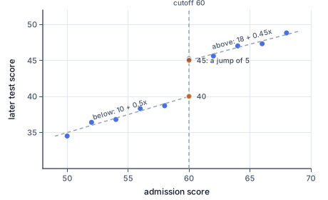
The figure plots this case: the two fitted lines meet the cutoff at 40 and 45, and the gap between them is the effect.
A selective school admits students scoring $60$ or more. Near the cutoff, the fit below is $\hat y = 10 + 0.5x$ and the fit above is $\hat y = 18 + 0.45x$, where $y$ is a later test score.
Three checks.
Then report the balance and density checks, and state that the effect is local to the cutoff.
Economics graduates earn more than most other graduates, but students who choose economics differ in many ways from those who do not. At the University of California, Santa Cruz, students could major in economics only if their grade point average in the introductory courses reached $2.8$. Students with $2.79$ and $2.81$ are very similar, but one group could declare the major and the other mostly could not.
Zachary Bleemer and Aashish Mehta used that cutoff as a regression discontinuity. Crossing $2.8$ sharply raised the probability of majoring in economics, and early-career earnings jumped at the same point. Scaling the earnings jump by the jump in majoring — a fuzzy RD — gave an effect of roughly $22{,}000$ dollars a year, about $46$ percent higher annual wages early in the career for students who majored in economics because they cleared the threshold.
The authors checked that students' backgrounds did not jump at $2.8$ and that grades did not bunch just above it. The estimate applies to students near the cutoff — those on the margin of being allowed into the major — which is exactly the group a university policy about grade thresholds affects, and the group a change in the cutoff would move into or out of the major.
The most common mistake is subtracting the two lines' intercepts when the running variable is not centered. The intercepts are values at zero, often far outside the data; the effect is the gap at the cutoff.
A second mistake is ignoring sorting. If people can place themselves just above the cutoff, those above differ from those below, and the jump is not an effect.
A third is generalizing the estimate. RD tells you the effect for units at the threshold.
Center the running variable.
$r = x - c$
Cutoff at zero.
Read the left fit.
$\hat y = 48 + 0.3r$
Below the cutoff.
Read the right fit.
$\hat y = 53 + 0.3r$
Above the cutoff.
Evaluate both at zero.
$48 \text{ and } 53$
The intercepts.
Subtract left from right.
$53 - 48 = 5$
The RD effect.
Read the cutoff.
$c = 50$
Treatment at 50 and above.
Read the left line.
$\hat y = 20 + 0.4x$
Below 50.
Evaluate it at the cutoff.
$20 + 0.4 \times 50 = 40$
Just below.
Read the right line.
$\hat y = 25 + 0.35x$
Above 50.
Evaluate it at the cutoff.
$25 + 0.35 \times 50 = 42.5$
Just above.
Subtract left from right.
$42.5 - 40 = 2.5$
Not $25 - 20 = 5$.
Read the outcome jump.
$\Delta y = 3$
At the cutoff.
Read the treatment jump.
$\Delta P(D=1) = 0.5$
Only half switch.
Recognize the design.
$\text{fuzzy RD}$
Probability, not certainty.
Divide the two jumps.
$3 \div 0.5 = 6$
Effect for compliers.
Compare with the outcome jump.
$6 > 3$
Dilution undone.
Name the group.
$\text{compliers at the cutoff}$
Local, and compliers only.
Name the assumption.
$\text{cutoff affects } y \text{ only via } D$
The exclusion restriction.
Evaluate the left fit.
$12 + 0.3 \times 40 = 24$
Just below.
Evaluate the right fit.
$10 + 0.4 \times 40 = 26$
Just above.
Subtract left from right.
With the running variable centered at the cutoff ($r = x - c$), a line fitted below the cutoff is $\hat y = 53 + 0.4r$ and one fitted above it is $\hat y = 56 + 0.4r$. What is the estimated jump at the cutoff?
Answer: jump at the cutoff
Complete the worked solution: with $r = x - c$, the left fit is $\hat y = 36 + 0.2r$ and the right fit is $\hat y = 44 + 0.2r$. Find the left and right values at $r = 0$, and the right fit's value $6$ units above the cutoff.
Evaluate the left fit at zero.
$\hat y_L(0) =$ a
Just below the cutoff.
Evaluate the right fit at zero.
$\hat y_R(0) =$ b
Just above the cutoff.
Evaluate the right fit further out.
$\hat y_R(6) =$ c
Away from the cutoff, the slope matters too.
The cutoff is $80$. Below it the fitted line is $\hat y = 30 + 0.2x$; above it, $\hat y = 28 + 0.25x$. Fill in each line's value at the cutoff.
Left line at the cutoff: yl. Right line at the cutoff: yr.
At a scholarship cutoff, the outcome jumps by $0.8$ and the probability of receiving the scholarship jumps by $0.2$. Fill in the outcome jump, the treatment jump and the fuzzy RD effect.
| value | |
|---|---|
| outcome jump | |
| treatment jump | |
| fuzzy RD effect |
A study uses a 3.0 GPA cutoff for a merit scholarship. Match each finding or worry to what it means for the RD design.
| sign of sorting: units near the cutoff may differ | another treatment at the same cutoff | RD estimates a local effect at the cutoff | reassuring balance check | |
|---|---|---|---|---|
| far more students have GPAs of 3.00 than 2.99 | ||||
| a 3.0 GPA also qualifies students for an honors dorm | ||||
| the scholarship's effect on 2.0 students is unknown | ||||
| family income is smooth across the cutoff |
Students scoring at least $65$ on an entrance exam are admitted to a selective high school. Using students near the cutoff, a line fitted below it is $\hat y = 8 + 0.4x$ and a line fitted above it is $\hat y = 20 + 0.3x$, where $y$ is a later test score and $x$ the entrance score. What is the estimated effect of admission at the cutoff?
Answer: test points
A university lets students major in economics only if their grade in the introductory courses reaches a cutoff. Crossing the cutoff raises the probability of majoring in economics by $0.2$, and early-career wages jump by $0.8$ thousand dollars at the cutoff. What is the effect of the economics major on wages for students at the cutoff, in thousand dollars?
Answer: thousand dollars
Lesson test: one question per skill, one attempt each, no hints. Your answers are checked when you submit.
At a scholarship cutoff, the outcome jumps by $1.2$ and the probability of receiving the scholarship jumps by $0.3$. Fill in the outcome jump, the treatment jump and the fuzzy RD effect.
| value | |
|---|---|
| outcome jump | |
| treatment jump | |
| fuzzy RD effect |
You can use a cutoff as a natural experiment. Explain to someone why bunching just above a cutoff undermines an RD estimate.
16. Your turn: cutoff 40; left fit y = 12 + 0.3x, right fit y = 10 + 0.4x., step 3
$26 - 24 = 2$
The RD effect.