Back to the on-screen lesson ·
Autocorrelated errors leave OLS unbiased but its standard errors wrong; the same persistence powers AR forecasts that head to a long-run mean and are judged by RMSE.
Paper packet. Every task here also exists on screen, where it is checked automatically; answers written on paper are not assessed by Nydus. When you are back at a device, enter your answers there.
By the end of this lesson you will be able to forecast from an AR(1) model one and two steps ahead, find its long-run mean, measure forecast accuracy, and diagnose serial correlation.
From the last lesson you know how to read trends and lags in time series. From the heteroskedasticity lesson you know that when an error assumption fails, OLS coefficients can remain unbiased while their standard errors go wrong, and that robust standard errors fix inference.
Time series bring one more error problem and one new task. The problem: errors in adjacent periods are usually related. The task: forecasting, which uses exactly that persistence to predict what comes next. This lesson treats both, and ends the course where much applied economics begins — with a forecast that has an honest measure of its accuracy.
| Term | What it means |
|---|---|
| Serial correlation | Correlation between a series' values, or a regression's errors, in different periods. |
| Autoregression | A regression of a series on its own past values; AR(1) uses one lag. |
| Persistence | $\rho$ in an AR(1): how much of this period's value carries into the next. |
| Long-run mean | $\mu = c/(1 - \rho)$: the level an AR(1) returns to when $\vert \rho\vert < 1$. |
| Forecast error | The actual value minus the forecast made for it. |
| RMSE | Root mean squared forecast error: the typical size of a miss, in the series' units. |
| HAC standard errors | Standard errors robust to heteroskedasticity and autocorrelation, such as Newey-West. |
Serial correlation. In a time-series regression $y_t = \beta_0 + \beta_1 x_t + u_t$, the errors often follow $u_t = \rho u_{t-1} + e_t$: a good quarter tends to be followed by another. If the regressors are strictly exogenous, OLS is still unbiased. But the usual standard errors assume the errors are independent. With positive $\rho$ the errors form runs, the data contain less independent information than their count suggests, and the usual standard errors are too small. HAC (Newey-West) standard errors correct them, much as robust errors corrected heteroskedasticity.
The Durbin-Watson statistic tests for first-order serial correlation in the residuals: $DW \approx 2(1 - \hat\rho)$, so values near $2$ mean little correlation and values near $0$ mean strong positive correlation.
Forecasting. Persistence is also what makes the future predictable. An AR(1) model $y_t = c + \rho y_{t-1} + e_t$ gives forecasts
$$\hat y_{T+1} = c + \rho y_T, \qquad \hat y_{T+2} = c + \rho \hat y_{T+1}, \qquad \hat y_{T+h} \to \mu = \frac{c}{1 - \rho}.$$
Each step closes a fraction $1 - \rho$ of the gap between the forecast and the long-run mean. Forecast accuracy is judged out of sample, by the root mean squared error of past forecasts.
Another way: action
Plot a regression's residuals in time order. If they run in long stretches above and below zero rather than bouncing randomly, they are positively serially correlated.
Another way: steps
Suppose the errors are strongly positively correlated: once the series is above the fitted line, it stays above for many periods. Ten years of monthly data then contain not $120$ independent pieces of information but something closer to a handful of long swings. The usual formula treats each month as independent and so overstates how much the data pin down the slope.
The result is standard errors that are too small, t statistics that are too large, and confidence intervals that are too narrow. Economists therefore report HAC standard errors for time-series regressions as a matter of course. The coefficient does not change; only the inference does, just as with heteroskedasticity.
A more serious problem arises when a lagged dependent variable is a regressor and the errors are serially correlated: then $y_{t-1}$ is correlated with $u_t$, and OLS is biased. Adding enough lags to make the remaining errors uncorrelated is the usual remedy.
In an AR(1) with $|\rho| < 1$, a series above its mean is pulled back toward it: each period, only a fraction $\rho$ of the deviation survives. Forecasting further ahead applies that shrinkage repeatedly, so the $h$-step forecast's deviation from the mean is $\rho^h$ times today's. As $h$ grows, $\rho^h$ shrinks to zero and the forecast approaches $\mu = c/(1 - \rho)$.
Persistence decides how fast. With $\rho = 0.25$, three-quarters of any deviation vanishes each period and forecasts reach the mean almost at once. With $\rho = 0.9$, only a tenth vanishes each period, so a high unemployment rate is forecast to stay high for years. Series with $\rho = 1$ — random walks — never return to any mean, and their best forecast is simply today's value.
A model that fits past data closely can still forecast badly, because it may have fitted noise. The honest test uses forecasts made with information available at the time: fit the model on data up to a date, forecast the next period, record the error, move forward one period, and repeat. The root mean squared forecast error of those out-of-sample forecasts measures typical accuracy in the series' own units.
Comparing RMSEs is how forecasters choose between models. A simple AR(1) often beats an elaborate model with many regressors out of sample, because the elaborate one chases noise. A useful benchmark is the naive forecast that next period equals this period; a model that cannot beat it is not worth its complexity.
Forecast uncertainty also grows with the horizon, because shocks accumulate. A careful forecast reports a band, not just a point, and the band widens the further out it goes. A forecast of next quarter's inflation might carry a band of half a percentage point; a forecast two years out, several points. Presenting only the center of a distant forecast gives it an authority the data cannot support, and readers deserve to see how much could plausibly differ.
Much of this course has been about causal questions: what would happen if $x$ changed. Forecasting asks a different question — what will happen, given everything known now — and uses different standards. A variable that predicts well need not cause anything; a forecast model needs no exclusion restriction and no parallel trends.
The distinction matters in practice. Rising stock prices may forecast recessions poorly while umbrella sales forecast rain well; neither says anything about what would happen if the variable were changed by policy. Economists sometimes speak of Granger causality, meaning that past values of $x$ improve forecasts of $y$. It is a statement about prediction, not about the effect of an intervention, and confusing the two is a common error in reading time-series results.
This lesson closes a sequence that began with a single question: what would happen if one thing changed and nothing else did? Every tool since has been an answer to part of it. Regression summarizes conditional means; its standard errors measure sampling uncertainty; controls, instruments, panels, differences-in-differences and discontinuities each remove a particular kind of selection bias under a particular assumption; time-series methods handle data that arrive in order.
The habits matter more than any single formula. State the question first, and say whether it is descriptive, predictive or causal. Name the comparison the method makes and the assumption that makes it credible. Check what can be checked — balance, pre-trends, first-stage strength, sorting at a cutoff — and argue what cannot. Report estimates with their intervals and their scope, and let the reader see the alternatives you considered.
From here, further study branches: more flexible models for nonlinear and limited outcomes, methods for many regressors, synthetic controls and modern difference-in-differences, structural models that combine economic theory with estimation, and machine learning for prediction. Each builds on the ideas of this course, and each is judged by the same standard: does it answer the question that was asked, and would a skeptic be persuaded?
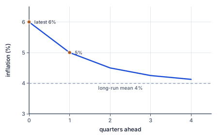
The figure plots these forecasts closing in on the long-run mean.
Quarterly inflation follows $\hat y_t = 2 + 0.5 y_{t-1}$, and the latest value is $6$ percent.
Three checks.
For regressions, check the residuals in time order and use HAC standard errors when they are autocorrelated.
Every month the Bureau of Labor Statistics reports the unemployment rate, and forecasters at the Federal Reserve, state agencies and banks predict where it is heading. The rate is highly persistent: an AR(1) fitted to monthly US data gives $\rho$ near $0.97$, so a rate that jumps in a recession is forecast to fall only slowly.
Take a stylized model $\hat u_t = 0.15 + 0.97\,u_{t-1}$, with a long-run mean of $0.15/0.03 = 5$ percent. If unemployment is $8$ percent, next month's forecast is $0.15 + 0.97 \times 8 = 7.91$ percent, and the gap to $5$ shrinks by only three percent each month. Forecasting a return to normal takes years, which matches the slow recoveries after the 1981 and 2008 recessions.
Forecasters judge such models by their out-of-sample RMSE and routinely find that simple autoregressions are hard to beat a few months ahead. Around turning points — the start of a recession — every model misses badly, which is why forecasts come with widening bands. Knowing how wrong a forecast has typically been is as important as the forecast itself. The Federal Reserve publishes its own projections with ranges for exactly this reason, so readers can see how wide the uncertainty really is.
The most common mistake is to think autocorrelated errors make OLS coefficients wrong. With strictly exogenous regressors they remain unbiased; the usual standard errors are what fail.
A second mistake is forecasting two steps ahead by plugging in today's value twice. The two-step forecast uses the one-step forecast as its input.
A third is judging a forecasting model by in-sample fit. Only forecasts made without seeing the outcome show how the model will perform.
Write the model.
$\hat y_t = 3 + 0.4 y_{t-1}$
An AR(1).
Read the latest value.
$y_T = 10$
This period.
Multiply by the persistence.
$0.4 \times 10 = 4$
Carried-over part.
Add the constant.
$3 + 4 = 7$
Next period's forecast.
Compare with the mean.
$\mu = 3 \div 0.6 = 5$
The forecast moved toward it.
Read the statistic.
$DW = 0.6$
From regression output.
Use the approximation.
$DW \approx 2(1 - \hat\rho)$
Links DW to residual correlation.
Halve the statistic.
$0.6 \div 2 = 0.3$
One step of the algebra.
Subtract from one.
$\hat\rho = 1 - 0.3 = 0.7$
Strong positive correlation.
Draw the consequence.
$\text{usual SEs too small}$
Errors run in streaks.
Apply the fix.
$\text{use Newey-West SEs}$
Coefficients unchanged.
List the forecast errors.
$0, 3, -4, 0$
Four quarters.
Square each error.
$0, 9, 16, 0$
Big misses count most.
Add the squares.
$25$
Sum of squared errors.
Divide by the count.
$25 \div 4 = 6.25$
Mean squared error.
Take the square root.
$\sqrt{6.25} = 2.5$
RMSE in the series' units.
Compare with a benchmark.
$\text{naive RMSE} = 3$
The model beats no-change.
Decide which model to keep.
$\text{keep the model}$
It forecasts better out of sample.
Forecast one step.
$1 + 0.8 \times 10 = 9$
Next period.
Forecast two steps.
$1 + 0.8 \times 9 = 8.2$
Uses the first forecast.
Find the long-run mean.
Monthly sales (thousands of units) follow $\hat y_t = 4 + 0.4\,y_{t-1}$. This month's sales were $30$ thousand. What is next month's forecast?
Answer: thousand units
Complete the worked solution: a regression's Durbin-Watson statistic is $1.6$. Find half the statistic, the implied first-order residual autocorrelation, and that autocorrelation's distance from zero.
Divide the statistic by two.
$DW \div 2 =$ a
From DW ≈ 2(1 − ρ̂).
Subtract from one.
$\hat\rho = 1 - DW/2 =$ b
The residual autocorrelation.
Take its absolute value.
$|\hat\rho| =$ c
Near zero: little serial correlation; near one: strong.
An AR(1) model is $\hat y_t = 1 + 0.8\,y_{t-1}$ and the latest value is $10$. Fill in the one-step forecast and the long-run mean.
One-step forecast: f1. Long-run mean: mu.
A model's forecast errors over four quarters were $1, -2, -2, 4$. Fill in the sum of squared errors, the mean squared forecast error and the root mean squared error.
| value | |
|---|---|
| sum of squared errors | |
| mean squared error | |
| root mean squared error |
The residuals of a regression of monthly sales on advertising are strongly positively autocorrelated. Match each claim to a verdict.
| true | false | |
|---|---|---|
| The slope is unbiased if advertising is strictly exogenous. | ||
| The usual standard errors are reliable. | ||
| Newey-West standard errors give valid large-sample tests. | ||
| A Durbin-Watson statistic near 0.6 signals the problem. |
A quarterly inflation series follows the estimated AR(1) model $\hat y_t = 1 + 0.75\,y_{t-1}$. The latest observation is $y_T = 8$ percent. What is the forecast for two quarters ahead?
Answer: percent
A state labor agency models its monthly unemployment rate as $\hat u_t = 2 + 0.6\,u_{t-1}$ (percent). Last month's rate was $7.8$ percent. What is this month's forecast?
Answer: percent
Lesson test: one question per skill, one attempt each, no hints. Your answers are checked when you submit.
A model's forecast errors over four quarters were $3, -3, 3, -3$. Fill in the sum of squared errors, the mean squared forecast error and the root mean squared error.
| value | |
|---|---|
| sum of squared errors | |
| mean squared error | |
| root mean squared error |
You can forecast and check a time-series regression. Explain to someone why autocorrelated errors make the usual standard errors too small.
17. Your turn: AR(1) with c = 1, ρ = 0.8 and latest value 10., step 3
$1 \div 0.2 = 5$
Where forecasts head.