Back to the on-screen lesson ·
Price and quantity are set together, so OLS finds neither curve; a shifter of one curve traces out the other and identifies its slope.
Paper packet. Every task here also exists on screen, where it is checked automatically; answers written on paper are not assessed by Nydus. When you are back at a device, enter your answers there.
By the end of this lesson you will be able to solve a linear market for equilibrium, explain simultaneity bias, and estimate a demand slope from a supply shifter.
From microeconomics you know supply and demand: the market price and quantity are where the two curves cross. From the last lesson you know how an instrument recovers a causal slope when the regressor is correlated with the error.
This lesson brings the two together. Price and quantity are simultaneously determined: each observation is an equilibrium, the crossing of two curves that both move. A regression of quantity on price therefore estimates neither curve, and the fix is an instrument chosen by economic reasoning about which forces shift which curve.
| Term | What it means |
|---|---|
| Simultaneous equations | A system in which several variables are determined together, such as price and quantity. |
| Structural equation | An equation with a behavioral meaning, such as a demand curve. |
| Reduced form | Each endogenous variable written as a function of the exogenous shifters only. |
| Supply shifter | A variable that moves supply but not demand, such as weather for crops. |
| Demand shifter | A variable that moves demand but not supply, such as income or tastes. |
| Identification | Whether the data can reveal a structural parameter at all, however large the sample. |
| Order condition | An equation is identified only if at least as many shifters are excluded from it as it has endogenous regressors. |
Write demand and supply as
$$Q = A - bP + u_d, \qquad Q = C + dP + u_s.$$
Setting them equal gives the equilibrium price $P^ = (A - C + u_d - u_s)/(b + d)$. The price depends on both* error terms. A demand shock raises price and quantity together; a supply shock raises quantity and lowers price. A scatter of equilibria is a cloud produced by both kinds of shock, and an OLS line through it estimates neither $-b$ nor $d$, but a blend that depends on which shocks were larger.
Now suppose supply also depends on weather $W$, which does not enter demand: $Q = C + dP + gW + u_s$. When weather changes, supply shifts while demand stays put, so the market slides along the demand curve. The demand slope is the ratio of weather's effect on quantity to its effect on price:
$$-b = \frac{\Delta Q / \Delta W}{\Delta P / \Delta W}.$$
That is the IV estimate with weather as the instrument for price. Weather's exclusion from demand is the exclusion restriction, and it comes from economics, not from the data.
Another way: action
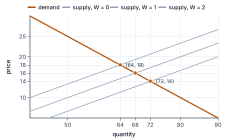
Draw a demand curve and several supply curves shifted by different weather. Mark where each crosses demand. The crossings all lie on the demand curve — connect them and you have drawn it.
Another way: steps
Take the demand equation $Q = A - bP + u_d$. OLS needs the price to be unrelated to $u_d$. But a positive demand shock raises the equilibrium price: $P^*$ contains $u_d/(b + d)$. So price and the demand error move together, and OLS is biased — the simultaneity bias.
The direction is predictable. Demand shocks push price and quantity up together, which makes the estimated demand curve too flat or even upward sloping. If demand shocks dominate, an OLS regression of quantity on price can give a positive slope and look like a supply curve. That is exactly what early economists found when they tried to estimate demand from market data, a puzzle that led to the modern theory of identification in the 1920s. The lesson those economists drew still holds: before asking how large a slope is, ask whether the data could possibly reveal it. A question about which curve is being traced has to be answered with economic reasoning about what moved, and only then with a regression. Without that reasoning, the most careful estimation is precise about a meaningless blend.
The figure shows the idea: as the weather shifts supply, the equilibria slide along the one demand curve and trace it out.
A variable that shifts only supply moves the equilibrium along a fixed demand curve. Every change it causes in price and quantity is a movement along demand, so their ratio is the demand slope. The shifter must satisfy the IV conditions: it must actually move supply (relevance) and must not enter demand (exclusion).
The same logic in reverse identifies supply: a demand shifter — income, a health report, a price change in a substitute — moves the market along a fixed supply curve.
The order condition counts: to identify an equation with one endogenous regressor (price), at least one shifter must be excluded from it and included in the other equation. If the only shifter moves both curves, neither is identified; the data cannot tell which curve moved.
Solving the system for price and quantity in terms of the shifters gives the reduced form: $P^ = \pi_0 + \pi_1 W + v_1$ and $Q^ = \gamma_0 + \gamma_1 W + v_2$. Each can be estimated by OLS, because $W$ is exogenous.
The reduced forms are useful for prediction — what happens to price when a frost hits — but they are not the behavioral curves. The structural demand slope is $\gamma_1/\pi_1$, a ratio of reduced-form coefficients. This is exactly the reduced form over first stage of the last lesson, with price as the endogenous regressor. Two-stage least squares does the same thing: regress price on weather, then quantity on predicted price.
Supply and demand are the classic case, but simultaneity appears wherever two variables cause each other. Police and crime: more crime leads cities to hire police, and more police reduce crime. Interest rates and output: the central bank responds to the economy, which responds to the central bank. Advertising and sales: firms advertise more when they expect strong sales.
In each case a regression of one on the other mixes the two directions of causation, and the remedy is the same: find a variable that moves one side for reasons outside the loop — election-year police hiring, an unexpected policy announcement, a change in advertising prices — and use it as an instrument. Each of those instruments has to meet the same two tests as weather in a fish market: it must move one side strongly, and it must have no path of its own to the other side. Where both tests are met, the loop is broken and a causal slope can be read off; where they are not, even a large and precise estimate describes only how the two variables happen to move together.
Why go to this trouble? Because demand slopes and elasticities answer practical questions that nothing else can. A state deciding whether to raise its cigarette tax needs to know how much smoking will fall and how much revenue will come in; both depend on the demand elasticity. An antitrust agency judging whether a merger will raise prices needs to know how easily buyers could switch to other products, which is a question about cross-price elasticities. A utility planning power plants needs to know how electricity use responds to price.
In each case an OLS regression on market data would mix the demand response with the supply response and could give an answer of the wrong size or even the wrong sign. A tax policy built on a demand curve that is really half a supply curve would badly misjudge both revenue and consumption.
That is why so much applied work in industrial organization, public finance and energy economics is organized around finding credible cost shifters for demand estimation and demand shifters for supply estimation. The econometrics is the instrumental-variables ratio; the economics is the argument that the shifter moves only one side of the market.
Demand is $Q = A - 2P$ and supply $Q = C + 3P + 10W$, where $W$ is good weather.
Three checks.
Then state the exclusion restriction in economic terms: why should weather not change how much buyers want at a given price?
Economist Kathryn Graddy recorded daily prices and quantities of whiting sold at New York's Fulton Fish Market in the early 1990s. A regression of quantity on price gives a muddled slope, because daily demand from restaurants and daily supply from boats both vary.
Weather at sea is the natural supply shifter. Stormy days keep boats in port and shrink the catch, but restaurants' menus do not change with the waves. Using stormy weather as an instrument for price, studies of these data find that stormy days raise the log price by roughly $0.3$ and lower the log quantity by roughly $0.35$, for a demand elasticity around $-1.1$: buyers cut purchases a bit more than proportionally when whiting becomes expensive.
The same design is used to estimate demand for electricity (with temperature shifting supply costs), for agricultural goods (with weather and disease), and for cigarettes (with state tax changes). In every case the credibility of the demand estimate rests on a claim about the market: that the shifter moves sellers and not buyers. For whiting, that claim is easy to believe; for many markets it takes real work to find a shifter that clean. Good studies show that the shifter does not predict demand-side variables such as buyers' incomes or the day of the week.
The most common mistake is regressing quantity on price and calling the slope demand. Market data are equilibria; without a shifter, the slope mixes supply and demand.
A second mistake is using a demand shifter to estimate demand. A variable that moves demand traces out supply.
A third is thinking the problem disappears with more data. Simultaneity is a problem of identification, not of sample size.
Write the two curves.
$Q = 40 - 2P, \ Q = 10 + 3P$
Demand and supply.
Set them equal.
$40 - 2P = 10 + 3P$
Same quantity at equilibrium.
Collect the terms.
$30 = 5P$
Price terms on one side.
Solve for the price.
$P^* = 6$
Where the curves cross.
Find the quantity.
$Q^* = 10 + 18 = 28$
Check: $40 - 12 = 28$.
Write the system.
$Q = A - P, \ Q = C + P + 6W$
Weather shifts supply.
Raise weather by one.
$\Delta W = 1$
Supply rises by 6.
Solve for the price change.
$\Delta P = -6 \div 2 = -3$
More supply, lower price.
Move along demand.
$\Delta Q = -1 \times (-3) = 3$
Demand did not move.
Divide the two changes.
$3 \div (-3) = -1$
The demand slope.
Check against the model.
$-b = -1$
Recovered exactly.
Suppose demand shocks dominate.
$Var(u_d) \gg Var(u_s)$
Tastes change a lot.
Trace a demand shock.
$u_d \uparrow \Rightarrow P \uparrow, Q \uparrow$
Along supply.
Look at the cloud.
$\text{points lie near the supply curve}$
Mostly supply is traced.
Run OLS of Q on P.
$\hat\beta > 0$
An upward slope.
Misread it as demand.
$\text{demand slopes up?}$
Nonsense.
Find a supply shifter.
$W = \text{weather}$
Moves the market along demand.
Use it as an instrument.
$\hat\beta_{IV} < 0$
The true demand slope.
Set the curves equal.
$50 - 3P = 10 + 2P$
Equilibrium.
Solve for the price.
$40 = 5P \Rightarrow P^* = 8$
Where they cross.
Find the quantity.
Demand is $Q = 68 - 4P$ and supply is $Q = 14 + 5P$. What is the equilibrium price?
Answer: dollars
Complete the worked solution: demand is $Q = 35 - 2P$ and supply is $Q = 23 + 2P$. Find the intercept gap, the equilibrium price and the equilibrium quantity.
Subtract the intercepts.
$35 - 23 =$ a
How far apart the curves start.
Divide by the sum of the slopes.
$P^* = \text{gap} \div (2 + 2) =$ b
Where the curves meet.
Put the price into supply.
$Q^ = 23 + 2P^ =$ c
The equilibrium quantity.
Demand is $Q = 84 - 4P$ and supply is $Q = 28 + 4P$. Fill in the equilibrium price and quantity.
Equilibrium price: p. Equilibrium quantity: q.
Demand is $Q = A - 0.5P$ and supply is $Q = C + 1.5P + 4W$, where $W$ is a weather index. If $W$ rises by one, fill in the change in price, the change in quantity and the ratio $\Delta Q / \Delta P$.
| value | |
|---|---|
| change in price | |
| change in quantity | |
| ratio ΔQ/ΔP |
In a market for coffee, match each shifter to what it lets you estimate. Frost in Brazil affects growers only; a health report praising coffee affects buyers only.
| identifies the demand curve | identifies the supply curve | identifies neither curve on its own | |
|---|---|---|---|
| frost in coffee-growing regions | |||
| a widely reported health study praising coffee | |||
| a variable that shifts both curves | |||
| no shifter at all, only price and quantity data |
In a market for strawberries, a spell of good weather raises supply. Comparing good-weather weeks with others, the price is $-2$ dollars per crate different and the quantity sold is $6$ thousand crates different. Weather does not affect how many strawberries buyers want at a given price. What is the slope of the demand curve, in thousand crates per dollar?
Answer: thousand crates per dollar
At New York's Fulton Fish Market, stormy days at sea cut the catch. On stormy days, the log price of whiting is $0.1$ higher and the log quantity sold is $0.14$ lower than on calm days. Storms do not change what restaurants want to buy at a given price. What is the price elasticity of demand?
Answer: elasticity
Lesson test: one question per skill, one attempt each, no hints. Your answers are checked when you submit.
Demand is $Q = A - 4P$ and supply is $Q = C + 2P + 12W$, where $W$ is a weather index. If $W$ rises by one, fill in the change in price, the change in quantity and the ratio $\Delta Q / \Delta P$.
| value | |
|---|---|
| change in price | |
| change in quantity | |
| ratio ΔQ/ΔP |
You can identify a curve from market data. Explain to someone why weather can reveal a demand curve but not a supply curve.
17. Your turn: demand Q = 50 − 3P, supply Q = 10 + 2P., step 3
$Q^* = 10 + 16 = 26$
Check: $50 - 24 = 26$.