Back to the on-screen lesson ·
Compute growth rates and trends, remove seasonality, read distributed-lag multipliers, and avoid spurious regressions between trending series.
Paper packet. Every task here also exists on screen, where it is checked automatically; answers written on paper are not assessed by Nydus. When you are back at a device, enter your answers there.
By the end of this lesson you will be able to compute growth rates and trend predictions, read impact and long-run multipliers, and recognize a spurious regression.
Every regression so far has used cross-sections — many units at one time — or panels. From the functional-form lesson you know that a log slope is a percent change, and from the omitted-variable lesson you know that anything moving with the regressor and the outcome can bias a slope.
Time-series data follow one unit — an economy, a firm, a market — through time: quarterly GDP, monthly unemployment, daily prices. The order of observations now matters. This lesson introduces the three features every time series must be checked for: trends, seasonal patterns and effects that take time to arrive.
| Term | What it means |
|---|---|
| Time series | Observations on one unit at successive dates, $y_1, y_2, \dots, y_T$. |
| Lag | An earlier value of a variable: $z_{t-1}$ is last period's $z$. |
| Distributed-lag model | A regression of $y_t$ on current and lagged values of $z$. |
| Impact multiplier | The coefficient on $z_t$: the same-period effect of a change in $z$. |
| Long-run multiplier | The sum of all the lag coefficients: the total effect of a permanent change. |
| Trend | A systematic rise or fall over time, often modeled as $\beta t$ or, in logs, as constant growth. |
| Spurious regression | A misleadingly strong relationship between series that share a trend but are otherwise unrelated. |
Trends. Many economic series grow over time. A linear trend $y_t = \alpha + \beta t + u_t$ adds $\beta$ each period; a log trend $\log y_t = \alpha + g t + u_t$ grows by about $100g$ percent each period. Growth rates are computed as the change divided by the earlier value.
Seasonality. Retail sales jump every December, construction slows every winter. Quarter or month dummies remove these calendar patterns, and year-over-year comparisons of the same season sidestep them.
Delays. A policy change may affect the outcome over several periods. A distributed-lag model captures that:
$$y_t = \alpha + \delta_0 z_t + \delta_1 z_{t-1} + \delta_2 z_{t-2} + u_t.$$
$\delta_0$ is the impact multiplier. After a permanent one-unit rise in $z$, the effect grows to $\delta_0 + \delta_1$ after one period and $\delta_0 + \delta_1 + \delta_2$ after two: that sum is the long-run multiplier. After a temporary one-period rise, the effects are $\delta_0$, then $\delta_1$, then $\delta_2$, and then zero.
Spurious regression. Two series that both trend will be highly correlated even if unrelated. Including a time trend, or regressing changes on changes, removes the common trend before relationships are read.
Another way: action
Plot a series over time. Look for a long-run slope (trend), a repeating pattern within each year (season), and a delayed response after known events (lags). Each needs its own treatment before a regression means anything.
Another way: steps
Suppose US cell-phone subscriptions and life expectancy both rose steadily from 1990 to 2020. A regression of one on the other gives a high $R^2$ and a very significant slope. But both simply rose over time for their own reasons; neither caused the other. The trend is an omitted variable that affects both series, and it moves perfectly with time.
The omitted-variable lesson gives the fix: include the omitted variable. Adding a time trend $t$ to the regression compares each series' deviations from its own trend. Alternatively, regress year-to-year changes on year-to-year changes; steady trends become constants and drop out. If the relationship survives detrending or differencing, it is at least not merely a shared trend.
Some series wander without a fixed trend at all — a random walk, whose changes are unpredictable. Regressions of one random walk on another are spurious in an even stronger way, and differencing is the standard remedy.
Suppose $z$ rises by one unit at time $0$ and stays there. At time $0$, only $z_t$ has changed, so $y$ rises by $\delta_0$. At time $1$, both $z_t$ and $z_{t-1}$ are one unit higher, so $y$ is $\delta_0 + \delta_1$ higher. At time $2$, all three terms are higher, and the effect is $\delta_0 + \delta_1 + \delta_2$. After that nothing new enters the model, so the effect stays there: the long run.
A temporary one-period change behaves differently: $z_t$ is high only at time $0$, so the effect is $\delta_0$ at time $0$, $\delta_1$ at time $1$ as the high value moves into the first lag, $\delta_2$ at time $2$, and zero after. The lag coefficients trace the response to a one-time shock; their sum is the response to a permanent one.
Monthly or quarterly data usually carry a calendar pattern. Comparing December sales with November's would suggest a boom every year and a bust every January. Two standard fixes: include a dummy for each month or quarter (leaving one out, as in the dummy lesson), or compare each period with the same period a year earlier.
Year-over-year growth rates do the second automatically, which is why government statistics often report them. Official series are also published seasonally adjusted, with the typical calendar pattern removed, so that a rise in adjusted unemployment in December means more than the usual holiday effect. When using published data, always check which version you have. Mixing an adjusted series with an unadjusted one in the same regression produces seasonal patterns in the residuals that look like real effects. The same care applies to prices: nominal series grow with inflation, so most economic comparisons over time use real values, deflated by a price index, to avoid confusing rising prices with rising quantities. A wage that doubles while prices triple is a pay cut, whatever the nominal series shows on a chart. Deflate first, then compare.
The cross-section assumptions carry over with one change: the random-sampling assumption is replaced by conditions on how the series behave over time. For OLS to be unbiased, the error must be unrelated to the regressors in every period — past, present and future — which rules out feedback from $y$ to future $z$. Many economic series violate this: a central bank sets interest rates in response to past inflation, so the rate is not independent of past inflation shocks.
Under weaker conditions OLS is still consistent in large samples, provided the series are stable — their means and correlations do not drift without limit. That is why detrending and differencing matter: they turn wandering series into stable ones for which the usual tools work. The next lesson takes up the other common problem, errors that are correlated over time.
A distributed-lag model needs a choice of how many lags to include, and the choice matters. Too few, and effects that arrive late are missed, so the long-run multiplier is understated and the omitted lags sit in the error, possibly biasing the included ones. Too many, and each coefficient is estimated imprecisely, because successive values of $z$ are usually highly correlated with one another — the multicollinearity problem from the multiple-regression lesson.
A practical approach starts from economic reasoning about how long an effect could plausibly take: a month for a price change to reach a gasoline pump, several years for a change in schooling policy to reach wages. Then it checks whether adding another lag changes the long-run multiplier much and whether the extra lags are jointly significant with an F test.
Individual lag coefficients are often noisy and can even flip sign from one lag to the next. Their sum, the long-run multiplier, is usually much more precisely estimated than any one of them, because the correlation among the lags that blurs each separate coefficient cancels when they are added. Report the long-run multiplier with its own standard error, which software computes directly.
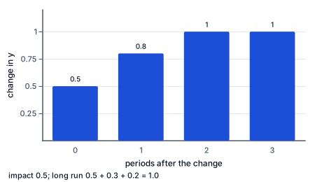
The bar chart shows this response period by period, building to the long-run multiplier.
In $y_t = \alpha + 0.5 z_t + 0.3 z_{t-1} + 0.2 z_{t-2} + u_t$, $z$ rises permanently by one unit at time $0$.
Half the long-run effect arrives at once; the rest takes two more periods.
Three checks.
And one reporting check: say whether the data are seasonally adjusted and whether growth rates are quarter-on-quarter or year-over-year.
When the Federal Reserve raises interest rates, inflation does not fall the next month. Economists estimate distributed-lag models of inflation on past interest-rate changes and find that the effects build over one to two years. A stylized result: a one-percentage-point rise in the policy rate lowers inflation by about $0.1$ points within a quarter, $0.3$ after four quarters and $0.5$ or more after eight.
Those numbers explain the Fed's saying that monetary policy works with "long and variable lags." A central bank that judged its policy by the impact multiplier would keep tightening long after it had done enough, because most of the effect of earlier moves had not yet arrived. The long-run multiplier, not the first-quarter response, is the number that matters for the total effect.
These estimates also illustrate the cautions of this lesson. Inflation and interest rates both trend over decades, so studies work with changes or detrended series; and the Fed sets rates in response to inflation, a feedback that simple regressions cannot untangle. Researchers therefore look for rate changes that were not responses to current conditions — surprises in policy announcements — much as the IV lesson recommends. Those surprise-based estimates confirm the long lags.
The most common mistake is reading a strong correlation between two trending series as evidence of a relationship. Almost any two series that grow over time will correlate.
A second mistake is reporting the impact multiplier as the total effect. When effects arrive over several periods, the long-run multiplier is the sum of all the lags.
A third is comparing adjacent months or quarters without accounting for seasonality. Compare the same season across years, or include season dummies.
Read the earlier value.
$y_{t-1} = 400$
Billions of dollars.
Read the later value.
$y_t = 412$
One year later.
Compute the change.
$412 - 400 = 12$
Billions.
Divide by the earlier value.
$12 \div 400 = 0.03$
Proportional change.
Convert to percent.
$3\%$
Annual growth.
Regress one trending series on another.
$R^2 = 0.95$
Looks strong.
Check both for trends.
$\text{both rise every year}$
A shared trend.
Add a time trend.
$y_t = \alpha + \beta x_t + \gamma t + u_t$
Controls for time.
Read the new slope.
$\hat\beta \approx 0$
No relation beyond the trend.
Try differences instead.
$\Delta y_t \text{ on } \Delta x_t$
Changes on changes.
State the conclusion.
$\text{spurious}$
The trend did all the work.
Write the model.
$y_t = \alpha + 2z_t + 1.5z_{t-1} + 0.5z_{t-2} + u_t$
Two lags.
Raise z permanently at time 0.
$\Delta z = 1$
And keep it there.
Read the effect at time 0.
$2$
Impact multiplier.
Add the first lag at time 1.
$2 + 1.5 = 3.5$
Cumulative.
Add the second lag at time 2.
$3.5 + 0.5 = 4$
Long-run multiplier.
Read it after time 2.
$4$
No further change.
Compare with a temporary change.
$2, 1.5, 0.5, 0$
Effects fade out.
Read the impact multiplier.
$0.2$
Same period.
Add the first lag.
$0.2 + 0.4 = 0.6$
After one period.
Add the second lag.
A country's real output was $400$ billion dollars last year and $412$ billion this year. What was its growth rate, in percent?
Answer: percent
Complete the worked solution: in $y_t = \alpha + 0.5\,z_t + 0.1\,z_{t-1} + 0.2\,z_{t-2} + u_t$, a permanent one-unit rise in $z$ starts at time $0$. Find the cumulative effect at time $1$, at time $2$, and the long-run multiplier.
Add the first lag to the impact.
$\text{time 1: } \delta_0 + \delta_1 =$ a
Two terms are now higher.
Add the second lag.
$\text{time 2: } \delta_0 + \delta_1 + \delta_2 =$ b
All three terms are now higher.
Name the long-run total.
$LRP =$ c
No further lags, so the effect stops growing.
A linear trend fitted to quarterly sales is $\hat y_t = 147 + 4t$. A log trend fitted to another series is $\widehat{\log y_t} = 3 + 0.0t$. Fill in the linear trend's prediction at $t = 10$ and the log series' growth rate per quarter in percent.
Linear trend at t = 10: lin. Growth per quarter: g percent.
In $y_t = \alpha + 0.2\,z_t + 0.4\,z_{t-1} + 0.1\,z_{t-2} + u_t$, $z$ rises permanently by one unit at time $0$. Fill in the effect on $y$ at times $0$, $1$ and $2$.
| effect on y | |
|---|---|
| time 0 | |
| time 1 | |
| time 2 |
Match each time-series finding to how it should be read.
| likely spurious: both just trend | seasonality: add quarter dummies | a relationship in changes, less prone to common trends | not evidence of a relationship by itself | |
|---|---|---|---|---|
| US cell-phone subscriptions and US life expectancy rose together for 30 years | ||||
| retail sales jump every fourth quarter | ||||
| year-to-year changes in interest rates predict changes in housing starts | ||||
| a high R-squared from regressing one trending series on another |
A finite distributed-lag model of monthly fertility on the real value of a child tax credit is $y_t = \alpha + 0.25\,z_t + 0.35\,z_{t-1} + 0.15\,z_{t-2} + u_t$. If the credit rises permanently by one unit, by how much does $y$ eventually rise?
Answer: long-run multiplier
A toy retailer's sales were $600$ thousand dollars in last year's fourth quarter and $648$ thousand in this year's fourth quarter. Sales always jump in the fourth quarter. What is the year-over-year growth rate for the fourth quarter, in percent?
Answer: percent a year
Lesson test: one question per skill, one attempt each, no hints. Your answers are checked when you submit.
In $y_t = \alpha + 0.2\,z_t + 0.4\,z_{t-1} + 0.1\,z_{t-2} + u_t$, $z$ rises permanently by one unit at time $0$. Fill in the effect on $y$ at times $0$, $1$ and $2$.
| effect on y | |
|---|---|
| time 0 | |
| time 1 | |
| time 2 |
You can work with time series. Explain to someone why two series that both grow over time can look related when they are not.
17. Your turn: coefficients 0.2, 0.4 and 0.1 on z_t, z_{t−1} and z_{t−2}., step 3
$0.6 + 0.1 = 0.7$
Long-run multiplier.