Back to the on-screen lesson ·
The assumptions that make OLS unbiased, the error variance with n − 2 degrees of freedom, and the slope's standard error from noise and spread.
Paper packet. Every task here also exists on screen, where it is checked automatically; answers written on paper are not assessed by Nydus. When you are back at a device, enter your answers there.
By the end of this lesson you will be able to state when OLS is unbiased, estimate the error variance, compute a slope's standard error, and predict how it changes with the sample.
You can fit a regression line and measure its fit. From statistics you know that a sample mean varies from sample to sample, with a standard error of $\sigma/\sqrt{n}$, and that this is what makes confidence intervals possible.
The OLS slope is also computed from a sample, so it varies too. This lesson asks two questions about that variation. Is the slope centered on the population slope — is it unbiased? And how spread out is it around that center — what is its standard error? The answers depend on a short list of assumptions, which the rest of the course will test one by one.
| Term | What it means |
|---|---|
| Unbiased | An estimator whose average over repeated samples equals the true parameter. |
| Sampling distribution | The distribution of an estimate across all possible samples. |
| Zero conditional mean | $E[u \mid x] = 0$: the error has the same mean at every value of $x$. |
| Homoskedasticity | $Var(u \mid x) = \sigma^2$: the error spread is the same at every $x$. |
| Error variance | $\sigma^2$, estimated by $\hat\sigma^2 = SSR/(n - 2)$. |
| Degrees of freedom | Observations minus estimated coefficients: $n - 2$ here. |
| Standard error | The estimated standard deviation of an estimator's sampling distribution. |
Write the population model as $y = \beta_0 + \beta_1 x + u$. Four assumptions make the OLS slope unbiased, $E[\hat\beta_1] = \beta_1$:
The fourth is the one that matters. It says nothing else that affects $y$ is systematically related to $x$ — which is exactly the absence of the selection bias from the first lesson. When it fails, the slope is biased however large the sample.
Add a fifth, homoskedasticity, $Var(u \mid x) = \sigma^2$, and the slope's sampling variance has a simple form:
$$Var(\hat\beta_1) = \frac{\sigma^2}{S_{xx}}, \qquad se(\hat\beta_1) = \frac{\hat\sigma}{\sqrt{S_{xx}}}, \qquad \hat\sigma^2 = \frac{SSR}{n - 2}.$$
Another way: action
Imagine drawing a hundred different samples of fifty workers and fitting the wage regression in each. The hundred slopes form a histogram. Unbiasedness is about where its center is; the standard error is about how wide it is.
Another way: steps
Substitute the population model into the slope formula. Because $\sum (x_i - \bar x) = 0$, the constant drops out and the slope becomes
$$\hat\beta_1 = \beta_1 + \frac{\sum (x_i - \bar x) u_i}{S_{xx}}.$$
The estimate is the truth plus a weighted sum of the errors. If the errors have mean zero at every value of $x$, the weighted sum has expected value zero for any given set of $x$'s, and so $E[\hat\beta_1] = \beta_1$.
Now suppose ability raises wages and is also higher among people with more schooling. Ability sits in $u$, and $u$ is then larger on average when $x$ is large. The weighted sum is systematically positive, and the slope overstates the return to schooling in every sample. No amount of data removes that: the bias is in the center of the histogram, not its width.
From the same expression, the slope's variation comes entirely from the weighted sum of errors. Each error has variance $\sigma^2$ under homoskedasticity, and the weights are $(x_i - \bar x)/S_{xx}$. The variance of the sum is $\sigma^2$ times the sum of squared weights, which works out to $\sigma^2 / S_{xx}$.
Each piece has an intuitive meaning. Noisier errors ($\sigma^2$ larger) make any one sample's slope wander further. More spread in $x$ ($S_{xx}$ larger) gives the line a longer lever: points far apart in $x$ pin down a slope more firmly than points bunched together. And because $S_{xx}$ grows roughly in proportion to $n$, the standard error shrinks with $\sqrt{n}$.
The spread lever is one a researcher can sometimes pull directly. An experiment that tests only two nearby doses of a drug learns little about the dose-response slope; one that tests doses far apart learns much more from the same number of patients. The same is true of a survey that deliberately includes workers with very little and very much schooling, rather than only the typical middle.
The residuals are not the true errors. OLS chose two coefficients to make the residuals as small as possible, so they are slightly smaller than the true errors on average, and the plain average of their squares would understate $\sigma^2$.
The two normal equations tie the residuals together: they must sum to zero and be uncorrelated with $x$. That leaves only $n - 2$ of them free to vary. Dividing by the number of free residuals, the degrees of freedom, corrects the understatement exactly and makes $\hat\sigma^2$ unbiased. With a hundred observations the correction barely matters; with ten, it matters a great deal.
The same logic extends to regressions with more coefficients. With $k$ regressors plus an intercept, OLS imposes $k + 1$ normal equations on the residuals, and the divisor becomes $n - k - 1$. You will meet that version in the lessons on multiple regression. It is also why a regression with nearly as many coefficients as observations is so unreliable: almost no degrees of freedom are left to measure the noise, and the estimated error variance itself becomes very uncertain, even before any question of bias arises.
Homoskedasticity says the errors are equally spread at every value of $x$. In wage data that is rarely true: wages of people with a high school diploma cluster fairly tightly, while wages of people with graduate degrees range from modest to enormous. The spread of the errors grows with schooling.
When that happens, two things are worth separating. The OLS slope is still unbiased, because unbiasedness needed only the first four assumptions. What breaks is the simple variance formula: $\sigma^2/S_{xx}$ assumed one $\sigma^2$ for everyone, and with unequal spreads the true variance is a weighted average in which observations far from the mean of $x$ count most. The usual standard error can then be too small or too large.
The fix, which a later lesson teaches, is a robust standard error that estimates the variance without assuming equal spreads. In practice most applied economists report robust standard errors by default. The formula in this lesson still matters, because it shows the levers — noise, spread, sample size — that drive precision under any assumption about the errors.
An estimator can be judged in two ways. Unbiasedness is about the average over many samples of a fixed size. Consistency is about what happens as a single sample grows: a consistent estimator gets closer and closer to the truth as $n$ increases.
Under the zero conditional mean assumption, OLS is both. Its standard error shrinks toward zero with more data, and its center is the true slope, so the estimates pile up on the truth. When the assumption fails, OLS is neither: its center is wrong, and more data only piles the estimates up on the wrong value. That is the precise sense in which big data cannot rescue a biased design, and it is why the second half of this course is about designs rather than sample sizes.
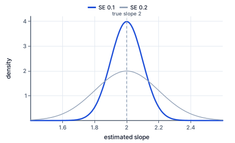
The figure shows what this standard error describes: the spread of the slope's sampling distribution, and how it doubles with a quarter of the spread in x.
A regression on $27$ students has $SSR = 100$ and $S_{xx} = 400$.
If the slope were $1.5$, a typical sample would give a slope within a few tenths of the truth — provided the zero conditional mean assumption holds, which the standard error itself cannot tell you.
Run three checks.
And one check of meaning: a standard error measures sampling variation only. It says nothing about whether the slope is biased.
The Current Population Survey interviews about $60{,}000$ US households every month, and much of what is known about wages comes from it. Why so many? Suppose a pilot study of $1{,}000$ workers finds a slope of $0.08$ in a log-wage regression on schooling, with a standard error of $0.012$. The estimate is precise enough to say schooling and wages move together.
Now suppose the question is narrower: does the return differ between two groups by one percentage point? To detect a difference that small, you want a standard error around $0.003$, a quarter of the pilot's. By the square-root law that needs sixteen times the data: about $16{,}000$ workers per group. Questions about small differences, subgroups or single states quickly demand tens of thousands of observations.
The same arithmetic warns against a common mistake. With the full survey, standard errors can be tiny, and almost every coefficient looks precise. But the zero conditional mean assumption is untouched by sample size. A precise estimate of the correlation between schooling and wages is still not the causal return to schooling unless ability and family background have been dealt with. A survey buys precision; only a research design can buy credibility for a causal claim.
The most common mistake is treating a small standard error as evidence that a slope is right. A standard error measures how much the estimate would vary across samples around its own center. If that center is biased, a small standard error only means the wrong answer is estimated precisely.
A second mistake is thinking more data fixes bias. Bias comes from the zero conditional mean assumption failing; it does not shrink with $n$.
A third is expecting the standard error to fall in proportion to the sample size. It falls with the square root: four times the data halves it.
Read the sample size.
$n = 52$
Observations.
Count the degrees of freedom.
$52 - 2 = 50$
Two coefficients estimated.
Read the residual sum.
$SSR = 450$
Squared misses added up.
Divide by the degrees of freedom.
$450/50 = 9$
The error variance.
Take the square root.
$\hat\sigma = 3$
A typical miss in the units of $y$.
Read the regression error.
$\hat\sigma = 5$
From SSR and $n - 2$.
Read the spread of x.
$S_{xx} = 100$
Sum of squared deviations.
Take its square root.
$\sqrt{100} = 10$
Back to units of $x$.
Divide the two numbers.
$5/10 = 0.5$
The slope's standard error.
Compare with the slope.
$\hat\beta_1 = 2.0$
Four standard errors from zero.
Interpret the standard error.
$\text{typical sampling error} \approx 0.5$
Not a measure of bias.
Start with the old sample.
$n = 200, \ se = 0.6$
One survey.
Quadruple the sample.
$n = 800$
Same population, same design.
Note how the spread grows.
$S_{xx} \times 4$
Proportional to $n$.
Note how its root grows.
$\sqrt{S_{xx}} \times 2$
Square root of four.
Keep the noise fixed.
$\hat\sigma \text{ unchanged}$
Same population.
Divide the old standard error.
$0.6/2 = 0.3$
Half as large.
Draw the lesson.
$\text{4× data} \Rightarrow \tfrac12 \text{ the error}$
Precision is expensive.
Divide by the degrees of freedom.
$400/16 = 25$
The error variance.
Take the square root.
$\hat\sigma = 5$
A typical miss.
Divide by the root of the spread.
A simple regression on $n = 29$ observations has a sum of squared residuals of $108$. What is the estimated error variance $\hat\sigma^2$?
Answer: error variance
Complete the worked solution: a regression on $30$ observations has $SSR = 448$ and $S_{xx} = 100$. Find the error variance, its square root and the slope's standard error.
Divide by the degrees of freedom.
$\hat\sigma^2 = 448 / 28 =$ a
Two coefficients used up two observations' worth.
Take the square root.
$\hat\sigma =$ b
Back in the units of $y$.
Divide by the root of the spread.
$se = \hat\sigma / \sqrt{100} =$ c
The slope's typical sampling error.
A regression's standard error is $\hat\sigma = 4$ and the regressor has $S_{xx} = 64$. What is the standard error of the slope?
Answer: standard error
With $200$ observations, a slope's standard error is $0.16$. If the survey is expanded to $800$ observations drawn the same way, about what standard error should the slope have?
Answer: standard error
A regression on $n = 27$ observations has $SSR = 100$ and $S_{xx} = 400$. Fill in $\hat\sigma^2$, $\hat\sigma$ and the slope's standard error.
| value | |
|---|---|
| error variance | |
| standard error of the regression | |
| standard error of the slope |
Match each change to its effect on the slope's standard error.
| the standard error rises | the standard error falls | |
|---|---|---|
| the outcome is measured with much more noise | ||
| the sample size doubles | ||
| the regressor varies over a wider range | ||
| every observation has almost the same x |
A state education department regresses district test scores on class size using $38$ districts. The regression leaves $SSR = 1296$, and class size has $S_{xx} = 400$. Assuming homoskedasticity, what is the standard error of the class-size slope?
Answer: points per student
Lesson test: one question per skill, one attempt each, no hints. Your answers are checked when you submit.
A regression on $n = 52$ observations has $SSR = 450$ and $S_{xx} = 225$. Fill in $\hat\sigma^2$, $\hat\sigma$ and the slope's standard error.
| value | |
|---|---|
| error variance | |
| standard error of the regression | |
| standard error of the slope |
You can measure an estimate's precision. Explain to someone why a huge sample can give a very precise estimate of the wrong number.
17. Your turn: n = 18, SSR = 400, S_xx = 100., step 3
$5/10 = 0.5$
The slope's standard error.