Back to the on-screen lesson ·
Read slopes in log-level, level-log and log-log models, rescale units, and find a quadratic's marginal effect and turning point.
Paper packet. Every task here also exists on screen, where it is checked automatically; answers written on paper are not assessed by Nydus. When you are back at a device, enter your answers there.
By the end of this lesson you will be able to read a coefficient under each log form, rescale it when units change, and compute a quadratic's marginal effect and turning point.
You can fit a line and read its slope in units of $y$ per unit of $x$. From algebra you know the natural logarithm and that $\log(ab) = \log a + \log b$; from calculus, that a derivative is a slope at a point.
Most relationships in economics are not straight lines in dollars. Wages grow in percentages, demand responds to percentage price changes, and earnings rise with experience and then flatten. This lesson shows how a linear regression can capture all of these by transforming the variables, and how to read each coefficient.
| Term | What it means |
|---|---|
| Log-level | $\log y$ on $x$: $100\beta$ is the approximate percent change in $y$ per unit of $x$. |
| Level-log | $y$ on $\log x$: $\beta/100$ is the change in $y$ per one percent change in $x$. |
| Log-log | $\log y$ on $\log x$: $\beta$ is an elasticity. |
| Elasticity | The percent change in one variable per one percent change in another. |
| Marginal effect | The change in the fitted $y$ for a small change in $x$: the derivative. |
| Turning point | The value of $x$ where a quadratic's marginal effect is zero. |
| Rescaling | Changing a variable's units, which rescales coefficients but not fit. |
OLS needs the model to be linear in its coefficients, not in the variables. So $\log(y) = \beta_0 + \beta_1 x$, $y = \beta_0 + \beta_1 \log x$ and $y = \beta_0 + \beta_1 x + \beta_2 x^2$ are all ordinary regressions: compute the new variable, then fit as before.
What changes is the reading. The key fact is that a small change in a natural log is approximately a proportional change: $\Delta \log y \approx \Delta y / y$. So:
With a squared term, the effect of $x$ changes with $x$: the marginal effect is $\beta_1 + 2\beta_2 x$, and if $\beta_2 < 0$ the curve peaks at $x^* = -\beta_1/(2\beta_2)$.
Another way: action
Take a wage of $20$ dollars and raise its log by $0.05$. The new wage is $20 e^{0.05} \approx 21.03$: about five percent higher. That is why a log coefficient reads as a percent.
Another way: steps
In $\log(y) = \beta_0 + \beta_1 x$, raising $x$ by one unit raises $\log y$ by exactly $\beta_1$. The ratio of new to old $y$ is then $e^{\beta_1}$, so the exact percent change is $100(e^{\beta_1} - 1)$.
For small $\beta_1$, $e^{\beta_1} \approx 1 + \beta_1$, and the percent change is close to $100\beta_1$. A slope of $0.08$ gives $8.3$ percent exactly and $8$ percent by the approximation, which is why economists read log coefficients directly as percents. For a coefficient of $0.5$, the exact change is $65$ percent, not $50$, and the exact formula should be used.
The same approximation works on the other side. A one percent rise in $x$ raises $\log x$ by about $0.01$, so in a level-log model it changes $y$ by $0.01\beta_1$, or $\beta_1/100$ units.
Measuring spending in cents instead of dollars multiplies every $y$ by $100$. Every fitted value and residual is multiplied by $100$ too, so the slope and intercept are $100$ times larger. Measuring income in thousands of dollars instead of dollars divides every $x$ by $1{,}000$; to predict the same $y$, the slope must be $1{,}000$ times larger.
None of this changes the fit: $R^2$ is identical, and so are $t$-statistics, as a later lesson shows. Rescaling is a choice about readability. A slope of $0.00004$ is correct and unreadable; the same slope as $4$ cents per thousand dollars is correct and clear. Logs remove the issue entirely, because a percent change is the same whatever the units.
Wages rise quickly early in a career and more slowly later. A regression on experience and experience squared captures that with a negative squared coefficient. The first coefficient alone is no longer "the effect of experience": it is the marginal effect at zero experience.
To report an effect, evaluate $\beta_1 + 2\beta_2 x$ at a meaningful value, such as the sample mean. The turning point $-\beta_1/(2\beta_2)$ is worth computing too. If it lies inside the data, the curve genuinely rises and then falls. If it lies far beyond the data — a peak at $80$ years of experience — the squared term is simply bending the line a little, and nobody should claim wages fall after the peak.
Which form should you use? Three questions usually settle it.
First, how does the outcome vary? Wages, prices, sales and populations are positive, skewed to the right and grow in proportions, so their logs are usually better behaved: the log of wages is close to symmetric even when wages themselves have a long upper tail. Test scores, temperatures and rates that can be zero or negative are left in levels.
Second, what question will be asked? A policy maker who wants to know the revenue from a tax needs dollars; one comparing responses across countries with different currencies wants elasticities, which a log-log model delivers directly.
Third, what does the picture show? Plot the conditional means, as in the second lesson. A curve that bends and flattens suggests a log on $x$ or a squared term; a fan that widens with $x$ suggests a log on $y$. Economic theory helps too: a production function with constant elasticities becomes exactly linear once both sides are logged.
Whatever the choice, say it plainly when reporting results. A reader who assumes levels when you used logs will misread every number in your table, and nothing in the table itself will warn them.
Logs have one practical catch: the log of zero is undefined, and the log of a negative number does not exist. Hours worked, charitable giving and trade between two countries are often exactly zero for many observations. Dropping those observations changes the sample and can bias the result, because the zeros are usually informative: they are the people who chose not to work, the donors who gave nothing.
Common fixes each come with a cost. Adding one before taking logs makes the coefficient depend on the units, which defeats the point of logs. Modeling whether the outcome is zero separately from how large it is when positive keeps the two questions apart, and a later lesson on binary outcomes gives the tools for the first half. The safe habit is to check how many zeros a variable has before choosing a log, and to say in the report what was done with them. A table of results that silently dropped a third of the sample is answering a question about a different population from the one the reader has in mind.
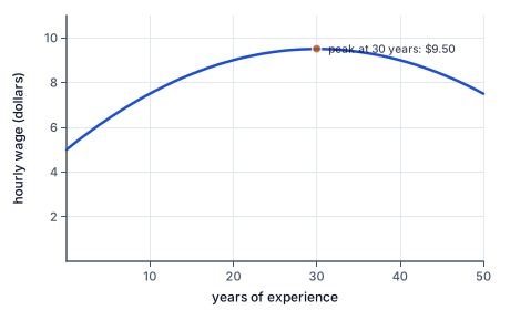
The figure draws this fitted wage curve, which peaks where the marginal effect reaches zero.
Take the fitted wage equation $\widehat{wage} = 5 + 0.30\,exper - 0.005\,exper^2$.
Reporting only the $0.30$ would overstate the effect of experience for almost everyone in the sample.
Run three checks.
For a quadratic, add a fourth check: at the turning point the marginal effect you compute must be zero.
Finally, read your sentence back as if you had never seen the regression. "Each extra year of schooling is associated with about eight percent higher wages" can be checked by anyone; "the coefficient is 0.08" cannot. Writing the answer in the units of the question is the check that catches the most misreadings, because a sentence that sounds absurd — wages eight cents higher per year of college — usually is.
How much less gasoline do Americans buy when the price rises? Economists regress the log of gasoline consumption on the log of its price, so the slope is directly an elasticity. Studies of US data typically find short-run elasticities between about $-0.03$ and $-0.3$: in the months after a price rise, people keep driving much as before. Long-run elasticities are larger, around $-0.3$ to $-0.8$, because over years people buy more efficient cars and move closer to work.
Put numbers on a policy. If a state tax raises pump prices by $10$ percent and the short-run elasticity is $-0.2$, consumption falls about $2$ percent at first. With a long-run elasticity of $-0.6$, it eventually falls about $6$ percent. That difference matters both for tax revenue, which holds up well in the short run, and for emissions, which fall more slowly than the long-run number suggests.
The log-log form makes these numbers comparable across states and decades, whatever the gallons or dollars involved, because an elasticity is unit-free. It also carries a warning for later: prices and quantities are set together by supply and demand, so a simple regression of one on the other needs care before its slope can be called a demand elasticity.
The most common mistake is reading $0.08$ in a log-wage regression as eight cents. It is a proportional change: about eight percent.
A second mistake is reporting the linear coefficient of a quadratic as the effect of $x$. With a squared term the effect varies with $x$ and must be evaluated at a stated value.
A third is thinking that rescaling a variable changes how well the model fits or how significant a coefficient is. It only moves the decimal point.
Identify the form.
$\log(wage) = \beta_0 + 0.08\,educ$
Log on $y$ only.
Apply the approximation.
$\%\Delta wage \approx 100 \times 0.08$
Per extra year.
State the approximate change.
$8\%$
Per year of schooling.
Compute the exact change.
$100(e^{0.08} - 1) \approx 8.3\%$
Close, because $0.08$ is small.
State it in words.
$\text{about 8 percent higher wage per year}$
A description, not yet a causal return.
Start from the original slope.
$0.05 \text{ dollars per dollar}$
Food spending on income.
Measure spending in cents.
$0.05 \times 100 = 5$
Every $y$ is 100 times larger.
Measure income in thousands.
$0.05 \times 1000 = 50$
One unit of $x$ is now 1000 dollars.
Do both at once.
$0.05 \times 100 \times 1000 = 5000$
Cents per thousand dollars.
Check the fit.
$R^2 \text{ unchanged}$
Rescaling never changes fit.
Pick the readable version.
$50 \text{ dollars per thousand}$
Same fact, easier to read.
Write the fitted equation.
$\hat y = 5 + 0.40x - 0.01x^2$
Wage on experience.
Differentiate the fitted equation.
$0.40 - 0.02x$
The marginal effect.
Evaluate at five years.
$0.40 - 0.10 = 0.30$
Dollars per extra year.
Evaluate at fifteen years.
$0.40 - 0.30 = 0.10$
The profile is flattening.
Set the effect to zero.
$0.40 - 0.02x = 0$
Find the peak.
Solve for the turning point.
$x^* = 20$
Years of experience.
Check inside the data.
$\text{workers with } x > 20 \text{ exist?}$
Otherwise the peak is extrapolated.
Recognize the elasticity.
$\beta_1 = -1.2$
Log on both sides.
Multiply by the price change.
$-1.2 \times 5 = -6$
Percent change in quantity.
State the result.
A regression of $\log(wage)$ on years of schooling has slope $0.03$. By about what percent is the fitted wage higher for each extra year of schooling?
Answer: percent
Complete the worked solution: a regression of weekly hours worked on $\log(wage)$ has slope $48$. Find the change in log wage for a $8$ percent rise, the resulting change in hours, and the change in hours per one percent.
Convert the rise into log points.
$\Delta \log(wage) = 8 / 100 =$ a
A small percent change is that many hundredths in logs.
Multiply by the slope.
$48 \times \Delta \log(wage) =$ b
Hours for the whole rise.
Find the change per percent.
$\beta_1 / 100 =$ c
The level-log reading of the slope.
A demand regression of $\log(quantity)$ on $\log(price)$ has slope $-0.3$. If the price rises by $8\%$, by about what percent does the fitted quantity change?
Answer: percent
A fitted earnings profile is $\hat y = 5 + 0.30x - 0.005x^2$, with $x$ in years of experience. At what experience does fitted earnings peak?
Answer: years
A regression of annual spending on food (in dollars) on annual income (in dollars) has slope $0.09$. Fill in the slope after each change of units.
| slope | |
|---|---|
| spending in cents, income in dollars | |
| spending in dollars, income in thousands of dollars | |
| spending and income both in thousands of dollars |
Match each model to how its slope $\beta_1$ is read.
| units of y per unit of x | about 100·b1 percent change in y per unit of x | about b1/100 units of y per 1% change in x | b1 percent change in y per 1% change in x | |
|---|---|---|---|---|
| y = b0 + b1 x | ||||
| log y = b0 + b1 x | ||||
| y = b0 + b1 log x | ||||
| log y = b0 + b1 log x |
Using monthly state data, an energy economist regresses $\log$ of gasoline consumption on $\log$ of the gasoline price and gets a slope of $-0.4$. A new state tax would raise pump prices by $11\%$. By about what percent would the fitted consumption change?
Answer: percent
Lesson test: one question per skill, one attempt each, no hints. Your answers are checked when you submit.
A regression of annual spending on food (in dollars) on annual income (in dollars) has slope $0.05$. Fill in the slope after each change of units.
| slope | |
|---|---|
| spending in cents, income in dollars | |
| spending in dollars, income in thousands of dollars | |
| spending and income both in thousands of dollars |
You can read a coefficient in any functional form. Explain to someone why 0.08 in a log-wage regression means eight percent, not eight cents.
17. Your turn: a log-log demand slope of -1.2 and a price rise of 5%., step 3
$\text{quantity falls about } 6\%$
Demand is elastic here.