Budgets and consumer choice

Paper packet. Every task here also exists on screen, where it is checked automatically; answers written on paper are not assessed by Nydus. When you are back at a device, enter your answers there.

1. What you will learn

You will derive a feasible consumer choice and check interior and corner conditions, showing the calculation and stating the assumptions that make the conclusion valid.

2. Starting point

Use the supplied definitions and units. Separate an accounting identity, a behavioral assumption, and a normative criterion before drawing conclusions.

3. Terms to use precisely

4. The feasible set and the objective do different jobs

Consumer choice combines a preference ordering with an opportunity set. A utility representation ranks bundles; a budget describes which bundles can be purchased at stated prices and income. A highly ranked but unaffordable bundle is not a feasible optimum. Conversely, an affordable bundle is not necessarily preferred to every other affordable bundle. The two ingredients must be analyzed together.

For two goods x and y with positive prices px and py and income m, the budget condition is px times x plus py times y no greater than m, with nonnegative quantities. This model assumes fixed prices, no borrowing beyond the stated budget, divisible goods, and no unlisted fees or quantity limits. Those conditions make the feasible set a triangle bounded by the axes and a straight budget line.

The single-good intercepts are m/px on the x axis and m/py on the y axis. They are alternative uses of the entire budget, not amounts that can both be purchased simultaneously. A bundle at both intercept quantities would require twice the income. The slope of the budget line is negative px/py, representing the market trade-off in y units per additional x.

The budget slope differs conceptually from the marginal rate of substitution. The price ratio describes what the consumer must give up in the market. The MRS describes what the consumer is locally willing to give up while remaining indifferent under the preference model. At a suitable smooth interior optimum, these rates coincide. Their equality is a conditional optimizing relationship, not a definition making preferences and prices the same thing.

Term	What it means
Budget set	Nonnegative bundles whose expenditure does not exceed the stated income.
Budget line	Bundles that spend the whole budget at given prices.
Interior optimum	A best feasible bundle with strictly positive quantities of both goods in this model.
Corner optimum	A best bundle with at least one choice at a boundary.
Tangency condition	Equality of a smooth local preference trade-off and the market trade-off under suitable interior conditions.
Demand function	A model's selected quantity as a function of its prices, income and other assumptions.

Another way: Derive an interior solution for the specified utility

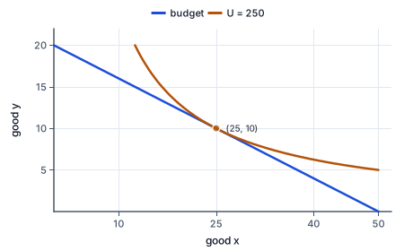
Good y against good x for a consumer with 100 dollars when x costs 2 and y costs 5. The budget line y = 20 − 0.4x runs from 50 x to 20 y. For utility U = xy, the highest indifference curve the budget reaches is xy = 250, touching the line at 25 x and 10 y, where half the budget goes to each good and the curve's slope equals the price ratio.

The figure shows the solution for one budget: the highest indifference curve the line reaches touches it where spending on the two goods is equal.

Take U(x,y)=xy with positive income and positive prices. On the strictly positive domain, both goods raise represented utility, so leaving spendable income unused cannot be optimal in this unconstrained two-good setting. The budget binds: px x+py y=m. The marginal utilities are y and x, making the MRS magnitude y/x.

At an interior solution, set y/x equal to px/py. Rearranging gives py y=px x: expenditure on the two goods is equal. Combining that condition with the binding budget gives px x=m/2 and py y=m/2. Thus x=m/(2px) and y=m/(2py). The equal expenditure shares follow from this equal-exponent product utility, not from a general law that consumers should split every budget in half.

The resulting quantities are positive because income and prices are positive. They satisfy the budget exactly, so the candidate is feasible and interior. To justify optimality, substitute the budget expression y=(m-px x)/py into U. The resulting function of x is a concave quadratic over the feasible interval, with its maximum at the derived x. This connects the consumer problem to the preceding optimization lesson.

Alternatively, a Lagrangian can combine U with the budget condition and nonnegativity constraints. The smooth interior first-order conditions equate marginal utility per unit of expenditure across the goods. The multiplier's numerical scale depends on the chosen utility representation, so it should not be presented as an objectively calibrated measure of happiness from money. The demand quantities and preference ranking, rather than arbitrary utility levels, carry the ordinal content.

Another way: Check the candidate against both resources and preferences

Suppose income is twenty-four, px three, and py two. The derived bundle is x four and y six. Its expenditure is three times four plus two times six, or twenty-four. Its MRS is six divided by four, or 1.5, matching the price ratio three divided by two. Its represented utility is twenty-four. Each check answers a different part of the optimization problem.

An affordable comparison bundle such as x two and y nine also spends twenty-four, but its product utility is eighteen. A bundle x six and y three spends the same amount and also yields eighteen. These comparisons illustrate why spending the entire budget does not by itself establish optimality. The chosen mix matters to the supplied preferences.

A bundle x five and y seven has product utility thirty-five but costs twenty-nine, exceeding the budget. Its higher utility is not evidence that the feasible optimum was calculated incorrectly. Optimization ranks feasible choices; it does not promise the best imaginable bundle regardless of resources. Explicitly checking expenditure prevents this common confusion.

Do not round continuous quantities before checking the budget unless the task specifies a rounding rule and an indivisible domain. If goods come only in whole units, evaluate the feasible integer alternatives near the continuous candidate and any relevant boundaries. A continuous solution remains useful as a guide, but an infeasible rounded bundle is not rescued by being close to the theoretical optimum.

Another way: Corners and kinks require different reasoning

The tangency method is not universal. Suppose utility is U=x+y, income twelve, px two, and py one. Each unit of either good adds one represented utility unit, but y provides more utility per dollar. The consumer buys y twelve and x zero. The optimum is a corner, and there is no feasible smooth interior point where the MRS of one equals the price ratio of two.

If the utility gain per dollar is equal for perfect substitutes, an entire set of budget-line bundles can be optimal. A question demanding one unique bundle would then need a tie rule. The absence of a unique solution is a feature of the stated preferences and prices, not a reason to force the equal-share formula onto a different utility function.

For perfect complements such as U=min(x,y), balanced quantities can be optimal because an unmatched extra unit does not improve utility. With positive prices and income, the budget and x=y condition give x=y=m/(px+py). The optimum is at a kink where a single smooth MRS may be undefined. A tangency calculation that differentiates through the kink without care would misrepresent the problem.

These examples show why a solution should identify the utility form, domain, and constraints before choosing a method. Interior first-order conditions, corner comparisons, and kink conditions are tools for different structures. The scored product-utility calculations explicitly stipulate their functional form, while the teaching explains how the reasoning would need to change under another model.

Another way: Demand responses are conditional comparative statics

Within the product-utility model, doubling income at unchanged prices doubles both selected quantities. Raising px while holding income and py fixed reduces x through m/(2px), while y remains m/(2py). These are comparative-static implications of this particular demand system. They do not establish that every consumer's demand for the other good is unaffected by a price change.

The price change also alters purchasing power. A lower price expands the budget set in a way that changes the relative price of the goods and the value of income in terms of available bundles. The next lesson separates these effects using a clearly defined compensated comparison. Simply observing that x rises after px falls does not identify how much is attributable to each channel.

The budget can also change through a quantity restriction or a borrowing limit rather than a price or income change. Such a restriction may make an otherwise derived product-utility bundle infeasible. Re-solve over the revised feasible set instead of treating the original demand formula as a rule immune to new constraints. A formula summarizes a solved model, including its assumptions.

Finish a consumer-choice reconstruction by reporting quantities, expenditure, and the relevant optimality check. State that the result follows from the supplied preferences, prices, income and divisibility. It is not financial advice, a claim that observed consumers calculate derivatives, or a statement that their welfare can be compared using raw utility levels. The model's value is to make the logic of constrained choice explicit and testable.

Another way: The dual question holds the target ranking fixed

The consumer problem maximizes represented utility for a given budget. A related expenditure-minimization problem asks for the least spending needed to reach a specified utility target at given prices. These are different questions with a useful connection: under suitable preferences and regularity conditions, the optimum of one can identify the target or budget for the other. In the numerical example, the bundle (4,6) reaches product utility twenty-four at expenditure twenty-four. A compensated comparison can later hold that target ordering fixed while prices change. The new expenditure needed to reach the target is not automatically the old income. This distinction prepares the income-and-substitution decomposition and prevents the word compensation from being used without saying what it preserves: an original bundle's affordability or an original utility level.

5. A fictional materials choice with two goods

A classroom consumer model represents a maker's preferences over paper units x and pigment units y by U=xy. The maker has twenty-four teaching-currency units, paper costs three per unit and pigment two. Quantities are divisible for this exercise, there are no additional fees, and the model includes no other goods or constraints. The task is to derive the best feasible bundle under those assumptions.

The budget intercepts are eight paper units and twelve pigment units. At a smooth interior optimum, the MRS y/x equals the price ratio 3/2. Combining that condition with the budget yields x four and y six. Expenditure is twelve on each good, totaling twenty-four, and represented utility is twenty-four. The equal spending pattern is a consequence of U=xy, not a universal budgeting recommendation.

The maker considers bundle (5,7), which has higher represented utility but costs twenty-nine. It is infeasible. Bundle (2,9) is affordable and spends all the income, but its utility is only eighteen. These comparisons distinguish two separate errors: ignoring affordability and assuming any budget-exhausting plan is optimal.

If paper's price falls to two while income and the pigment price remain fixed, the product-utility model chooses six units of each good. That is a new conditional prediction using changed prices. A real application would require evidence about preferences, available goods and other constraints before treating the formula as a behavioral forecast. Here the complete calculation shows how an ordinal objective and a budget jointly determine a feasible choice.

6. Check the tempting inference

A preferred bundle can be unaffordable; spending all income is not sufficient for optimality. The equal-share formula belongs to product utility, not every consumer. Interior tangency needs suitable smoothness and a feasible interior candidate; substitutes and complements can require corners or kinks. Utility multipliers inherit an arbitrary ordinal scale.

7. Derive a smooth interior bundle

8. A high-utility bundle can be infeasible

9. A different utility gives a corner

10. Finish a product-utility demand calculation

11. Guided practice

Maximize U=xy with income 24, px3, py2 and nonnegative divisible goods. Give optimal x,y and represented U; there are no other constraints.

12. Guided practice

Use U=xy, income 32, px4 and py2 with divisible nonnegative goods. Complete the interior demand calculation.

13. Guided practice

Use U=xy, income 48, px4 and py3, with positive divisible quantities and no other constraint. Give optimal x,y and represented U.

14. Practice

Plot the supplied budget-line combinations (x,y)=(0,12),(4,6),(8,0), with x horizontal and y vertical. These are quantities affordable with m24, px3 and py2. The middle point is the product-utility optimum.

15. Practice

A different preference model has U=x+y, income 12, price of x2 and price of y1, with nonnegative divisible quantities. Construct optimal x, optimal y and utility; the product-utility equal-share formula does not apply.

16. Somewhere new

A fictional maker is represented by U=xy over paper x and pigment y. The classroom budget is 36, px3 and py2; quantities are divisible and no other cost is included. Derive the optimal quantities and represented utility rather than recommending an actual purchase.

17. Lesson test

Lesson test: one question per skill, one attempt each, no hints. Your answers are checked when you submit.

18. Test question

A new product-utility model has U=xy, income 80, px5 and py4, with nonnegative divisible goods and no additional constraints. Give optimal x,y and represented U.

19. What you can do now

Reconstruct a fresh case without the worked solution. Explain which assumption would change its conclusion and which result is only an accounting or model condition.

	Your result
Optimal x
Optimal y
Represented U at the optimum