Derive cost measures and a bounded output choice while distinguishing fixed, avoidable and marginal costs.
Paper packet. Every task here also exists on screen, where it is checked automatically; answers written on paper are not assessed by Nydus. When you are back at a device, enter your answers there.
1. What you will learn
You will derive cost measures and a bounded output choice while distinguishing fixed, avoidable and marginal costs, showing the calculation and stating the assumptions that make the conclusion valid.
2. Starting point
Use the supplied definitions and units. Separate an accounting identity, a behavioral assumption, and a normative criterion before drawing conclusions.
3. Terms to use precisely
Term
What it means
Cost function
Minimum expenditure for output under specified technology, input prices and constraints.
Variable cost
The part of cost that changes with the selected output in the stated model.
Marginal cost
The local increase in cost from additional output.
Average cost
Total cost divided by positive output, distinct from marginal cost.
Shutdown
Zero current production while some fixed commitments can remain.
Exit
Leaving an activity over a horizon in which additional costs may become avoidable.
4. A cost function summarizes a production problem
A firm's cost function describes the least cost of producing each output quantity under a specified technology, input prices and set of adjustable inputs. It is not merely a list of past payments. A short-run function can hold some inputs fixed, while a long-run function permits a broader adjustment. The time horizon and constraints therefore belong to the definition of the model rather than being inferred from the word cost.
Suppose total short-run cost is C(q)=F+cq+dq squared for q at least zero, with d positive. F is a fixed cost that remains unavoidable during the current operating decision. The variable part is cq+dq squared. The linear term can represent a constant per-unit requirement, while the quadratic part captures rising resource requirements at the margin. These interpretations motivate a bounded model rather than establish that all firms have quadratic cost.
A production relation can generate such a shape. If output q requires labor L=q squared and labor costs d per unit, labor expense is dq squared. Adding a material cost c per output unit gives the stated variable cost. This derivation makes clear which technology and input-price assumptions support the curve. A change in wages, production methods or the set of adjustable inputs can change the function.
The fixed cost is a level term in this short-run account. It affects total cost and profit but not the derivative of variable cost with respect to output. That mathematical fact does not make fixed resources free or irrelevant to every decision. It means that, when F is unchanged across the current feasible quantities, it does not alter their incremental ranking. Entry, exit, or capacity investment can pose a different choice.
Another way: Keep total, average and marginal measures separate
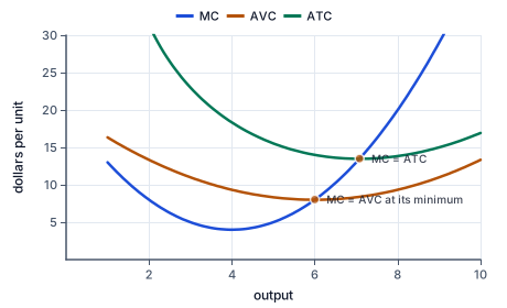
Dollars per unit against output for a firm with variable cost Q³/3 − 4Q² + 20Q and a fixed cost of 36. Marginal cost falls to its lowest at 4 units and then rises. It crosses average variable cost at that curve's minimum, 8 dollars at 6 units, and average total cost at its minimum, about 13.5 dollars near 7.1 units. The gap between the two averages is average fixed cost, which narrows as output grows.
The figure draws the three per-unit measures together: marginal cost crosses each average at its minimum.
Total cost C(q) is the cost of the whole selected output. Average total cost is C(q)/q for positive q. Average variable cost is VC(q)/q, equal to c+dq in this model. Marginal cost is the derivative C'(q)=c+2dq. These quantities answer different questions and have different behavior even though they come from one function.
For F twelve, c two, d one and q three, variable cost is six plus nine, or fifteen. Total cost is twenty-seven. Average total cost is nine, average variable cost five, and marginal cost eight. The marginal cost is the local cost of an additional small unit; it is not the average cost of the three units already produced. Replacing one with another would change the firm's optimizing condition.
At q zero, the ratios defining average cost are not defined. Total fixed cost can still be F, while variable cost is zero. Do not assign an arbitrary average cost of zero merely because no output is produced. A shutdown comparison should use total or avoidable costs directly rather than divide by a nonexistent output quantity.
The relationship between marginal and average values provides a check. If marginal cost is below an average cost measure, adding a small amount of output tends to pull that average down; if above, it tends to raise it. This is a mathematical relationship between a total and its average, not evidence that a firm always chooses the minimum average-cost quantity. Output choice also depends on the revenue available at different quantities.
Another way: A price-taking output decision compares price with marginal cost
For a price-taking firm facing fixed output price P, revenue is Pq. Profit in the short-run model is Pq-F-cq-dq squared. The marginal profit is P-c-2dq. An interior candidate therefore satisfies P=c+2dq, or price equals marginal cost. Because d is positive, profit is strictly concave in q, so a feasible stationary point is the unique maximum over the nonnegative continuous domain.
The unconstrained candidate is (P-c)/(2d). If P exceeds c, it is positive and gives the short-run operating quantity under the model. If P is below or equal to c, no positive quantity improves profit relative to q zero, so the firm shuts down production for the period. Its profit at q zero is negative F because the fixed cost remains unavoidable in this decision.
For P eight, c two and d one, the selected quantity is three. Variable cost is fifteen and revenue twenty-four. With F twelve, profit is negative three. The firm nevertheless loses less by producing than by shutting down and losing all twelve fixed-cost units. A negative total profit therefore does not automatically imply immediate shutdown when an unavoidable fixed cost is present.
The price-taking condition is an assumption about the firm's perceived revenue opportunity. If selling more requires reducing the price on all units, marginal revenue need not equal price and the same equation would be inappropriate. The market-power lesson changes that revenue side explicitly. Do not transfer P=MC to every market structure simply because it is familiar.
Another way: Shutdown and exit differ because avoidability differs
A short-run shutdown stops current output while unavoidable fixed commitments remain. Long-run exit can avoid costs that are fixed within the current period but no longer binding over a broader horizon. The decision rule changes when the alternative changes. A payment should not be treated as permanently sunk merely because it appears as F in one short-run equation.
In the preceding example, producing q three yields profit negative three while shutting down yields negative twelve. If a later exit option avoids the entire fixed cost and leaves a zero payoff, continuing the same operation at negative three would be worse than exiting under those unchanged values. This is not a contradiction. The short-run alternative was minus twelve; the long-run alternative is zero.
When a fixed setup charge is incurred only if production is positive, it is avoidable at q zero. Then the firm must compare the best positive-output profit with the zero-output payoff directly. The interior first-order condition can identify the best operating quantity but does not decide whether paying the setup charge is worthwhile. A global comparison across the discontinuity is needed.
Real adjustment can involve resale, contractual penalties, retraining, uncertainty and other consequences. Those features belong in the relevant alternatives if the model includes them. The lesson's simple account deliberately states what is unavoidable and what can be avoided. That clarity prevents a cost label from doing the work of an economic analysis that has not actually compared the options.
Another way: Input choice and the long-run envelope add another layer
A long-run cost problem can minimize expenditure over several input combinations capable of producing the target output. With smooth technology and an interior solution, the ratio of marginal products can be matched to the ratio of input prices. Corners, fixed proportions or indivisibilities can require a different method. As with consumer choice, a tangency condition is a tool with assumptions rather than a universal definition of optimality.
Allowing more input adjustment cannot raise the minimum cost of a given output if every old feasible input plan remains available and input prices are unchanged. The long-run minimum can match or improve on the restricted short-run cost. A graph often describes the long-run cost as an envelope of short-run possibilities. This statement is conditional on nested feasible sets, not a claim that observed long-run costs must fall when wages or technology also change.
Returns to scale describe how output changes when all inputs scale together. Diminishing marginal product of one input while another is fixed is a different concept. Confusing the two can lead to an unsupported claim that rising short-run marginal cost proves decreasing returns to scale. State which inputs change in the comparison and which remain fixed.
For each exercise, identify the horizon, the price-taking assumption, the nonnegative output domain and the fixed-cost treatment. Derive the operating quantity, calculate variable cost and revenue at that feasible quantity, and subtract the unavoidable F once. Then explain the comparison with shutdown. This complete account is more informative than either 'minimize cost' or 'produce where curves cross' without specifying the objective and available alternatives.
Another way: An input-price change changes the cost problem
If the wage changes, a previously cost-minimizing input combination need not remain optimal. With several substitutable inputs, the firm can substitute toward an input whose relative price falls. A cost comparison that holds the old input quantities fixed measures the expense of that old plan, not necessarily the new minimum cost. Locally, under the regularity conditions for the envelope theorem, the derivative of minimized cost with respect to an input price equals the conditional demand for that input. This result distinguishes the direct price effect from the reoptimization of quantities; it does not assume that technology or output demand also stays unchanged in a real wage shock.
5. A workshop operates at a short-run loss
A fictional workshop takes a price of eight teaching-currency units per output unit as given. Its stipulated short-run cost is twelve plus two q plus q squared. Output is continuous and nonnegative, and the twelve-unit fixed commitment cannot be avoided during the current period. No other capacity or market constraint is included.
Marginal cost is two plus two q. Equating it with price eight gives q three, and the negative second derivative of profit confirms a concave maximum. At q three, variable cost is six plus nine, or fifteen; revenue is twenty-four; total cost is twenty-seven; and profit is negative three. Reporting the loss is correct, but it does not complete the current operating comparison.
If the workshop produces nothing this period, variable cost and revenue are zero while the fixed twelve remains payable. Shutdown therefore gives profit negative twelve. Operating at negative three is better by nine under the stated short-run alternatives. The reason is that revenue covers variable cost and contributes toward the unavoidable commitment, not that a loss has somehow become a positive profit.
For a later period, suppose the workshop can exit and avoid the twelve-unit commitment entirely. The alternative payoff can then be zero, changing the comparison with continuing at negative three. A real decision would require the relevant future prices, adjustment costs and other facts. The exercise demonstrates why the horizon and avoidability of costs must be specified before using a negative-profit observation to recommend shutdown or exit.
6. Check the tempting inference
Marginal cost is not average cost, and a fixed cost is not automatically irrelevant to every decision. Negative operating profit does not alone imply short-run shutdown when F is unavoidable. An avoidable setup charge or a long-run exit option requires a global comparison with its own zero-output payoff. Price equals marginal revenue only under the price-taking assumption.
7. Separate the cost measures
State the cost function and output.
C=12+2q+q^2; q=3
The model separates a fixed commitment from variable requirements.
Calculate variable and total cost.
VC=6+9=15; C=27
Add F once after calculating variable cost.
Calculate average variable cost.
15/3=5
This ratio is defined because output is positive.
Calculate average total cost.
27/3=9
The fixed cost contributes four per unit at this quantity.
Calculate marginal cost separately.
MC=2+2x3=8
The local cost of another unit differs from both averages.
8. Find the price-taking operating quantity
State the price and current cost model.
P=8; C=12+2q+q^2
Price is held fixed as the firm changes output.
Differentiate profit with respect to output.
Marginal profit=8-2-2q
Unavoidable F has zero derivative.
Solve and check the interior candidate.
q=3; profit second derivative=-2
The positive quantity maximizes the concave objective.
Evaluate the current profit.
Revenue 24; VC15; F12; profit=-3
A maximum can still have a negative level.
Compare with zero output.
Shutdown profit=-12; operating improves by 9
The relevant short-run alternative still pays F.
9. Change the avoidability of the fixed commitment
Keep the operating calculation visible.
Best positive-output profit=-3
This is the result under the same price and technology.
Describe the original shutdown alternative.
q0 still costs 12
The commitment was unavoidable this period.
Introduce a different later-period alternative.
Exit avoids F and yields 0
The feasible economic consequences have changed.
Compare continuation with exit.
0>-3
Under the revised alternatives, exit dominates continued operation.
Explain why the earlier result was not inconsistent.
Short-run comparator=-12; later comparator=0
The decision horizon changes which costs can be avoided.
Name the information still needed in an application.
Future prices, adjustment costs and contractual conditions
A cost-function exercise is not a recommendation without its actual alternatives.
10. Finish an operating comparison
P10 and C8+2q+q^2 describe the current model.
q=(10-2)/2=4
The positive candidate maximizes concave profit.
Evaluate variable cost and revenue.
VC=8+16=24; revenue 40
Use the selected output in both expressions.
Your turn: work this step out. Its working is at the end of the packet.
Subtract the unavoidable commitment.
11. Guided practice
A price-taking firm faces P 10 and cost C(q)=12+2q+q^2 for continuousq>=0. F12 is unavoidable this period. Give optimal q, variable cost and profit.
Your result
Optimal current q
Variable cost at that q
Profit including unavoidable F
12. Guided practice
P12 and C(q)=10+2q+q^2 apply with an unavoidable fixed 10 and nonnegative continuous output. Complete the current operating calculation.
Solve price equals marginal cost and check feasibility.
q
Twelve equals two plus twice the chosen output.
Evaluate variable cost.
vc
Use two times output plus output squared, excluding the fixed commitment.
Calculate profit including the fixed cost once.
profit
Subtract variable cost and ten from twelve times output.
13. Guided practice
Use P 8 and C(q)=12+2q+q^2, with F 12 unavoidable and continuousq>=0. Give the current optimal q, variable cost and profit, even if profit is negative.
Optimal current q: v0. Variable cost at that q: v1. Profit including unavoidable F: v2.
14. Practice
Use P 2 and C(q)=9+4q+q^2. F9 is unavoidable; output is continuous and nonnegative. Give optimal q, variable cost and profit.
Optimal current q: v0. Variable cost at that q: v1. Profit including unavoidable F: v2.
15. Practice
Cost is C(q)=10+2q+q^2. At the supplied output q=5, construct total cost, average variable cost and marginal cost. The fixed 10 is unavoidable; do not confuse average and marginal measures.
Total cost: v0. Average variable cost: v1. Marginal cost: v2.
16. Somewhere new
A fictional workshop takes P 14 as given and has the stipulated short-run cost 20+2q+q^2. Its fixed 20 cannot be avoided this period. Reconstruct the optimal continuous output, variable cost and profit; no actual operating recommendation is requested.
Optimal current q: v0. Variable cost at that q: v1. Profit including unavoidable F: v2.
17. Lesson test
Lesson test: one question per skill, one attempt each, no hints. Your answers are checked when you submit.
18. Test question
A fresh price-taking model has P 20 and C(q)=18+4q+2q^2 for continuousq>=0. F18 remains payable if output is zero. Give the current optimum, its variable cost and total profit.
Optimal current q: v0. Variable cost at that q: v1. Profit including unavoidable F: v2.
19. What you can do now
Reconstruct a fresh case without the worked solution. Explain which assumption would change its conclusion and which result is only an accounting or model condition.
Working for the steps left to you
10. Finish an operating comparison, step 3
Profit 40-24-8=8
Shutdown would pay the same fixed eight with no revenue.