Derive a capital transition and bounded steady state under explicit saving and depreciation assumptions.
Paper packet. Every task here also exists on screen, where it is checked automatically; answers written on paper are not assessed by Nydus. When you are back at a device, enter your answers there.
1. What you will learn
You will derive a capital transition and bounded steady state under explicit saving and depreciation assumptions, showing the calculation and stating the assumptions that make the conclusion valid.
2. Starting point
Use the supplied definitions and units. Separate an accounting identity, a behavioral assumption, and a normative criterion before drawing conclusions.
3. Terms to use precisely
Term
What it means
Gross investment
Total new capital formation before subtracting depreciation.
Net accumulation
Investment minus depreciation under the stated stock equation.
Steady state
A stock level unchanged by the specified transition rule.
Capital dilution
Lower capital per worker caused by a growing worker denominator, other things equal.
Golden rule
The capital level maximizing sustainable steady-state consumption under the model.
Conditional convergence
A convergence comparison that holds the relevant determinants of the steady state fixed.
4. A capital stock changes through dated flows
Economic growth concerns changes in productive capacity and output over time. Before explaining those changes, distinguish a stock of productive equipment from a flow of newly produced investment. Capital K at the start of a period is available for that period's production. Investment during the period adds equipment for the next period, while depreciation removes part of the existing stock. Counting investment as though it were already the whole stock loses this timing.
Use a deliberately small closed-economy model with one good, a constant labor force, no government and no foreign borrowing. The good can be consumed or transformed into capital one for one. Let output per worker be y=A times the square root of k, where k is capital per worker and A is a positive fixed productivity parameter. Labor and productivity do not grow in the main numerical exercises.
A constant fraction s of output becomes investment, with s strictly between zero and one. A fraction delta of the current capital stock depreciates, with delta positive and no greater than one. The transition equation is next k=(1-delta)k+sA square root of k. It specifies the next stock rather than merely the change in the stock. Subtracting current k gives net accumulation sA square root of k minus delta k.
This saving rule is a behavioral assumption, not an accounting necessity that households always save the same fraction. The model does not derive s from preferences or institutions. Earlier intertemporal choice showed how preferences and constraints can determine saving. Holding s fixed here isolates a simpler mechanism: investment creates future capital, but more capital also requires more replacement investment.
Another way: Diminishing returns govern the transition
With y=A square root of k, increasing capital raises output at a diminishing marginal rate when labor is fixed. The derivative is A divided by twice the square root of k for positive k. Doubling capital does not double output: multiplying k by four doubles its square root. This is diminishing marginal product of capital, not a statement that all inputs have been scaled together.
The underlying aggregate production function can be Y=A square root of K times square root of L. Scaling both capital and labor by the same positive factor scales output by that factor, giving constant returns to scale. Dividing by L gives the stated per-worker function. Thus constant returns to scale and diminishing returns to capital per worker can coexist without contradiction.
Investment per worker sA square root of k rises as capital increases, but the replacement requirement delta k rises linearly. At low positive capital, investment can exceed depreciation and the stock grows. At high capital, depreciation can exceed investment and the stock contracts. The comparison concerns net accumulation, not whether investment is positive. A country can invest every period while its capital stock falls.
For A two, s one quarter, delta one eighth and k four, output is four and investment one. Depreciation is one half, so next capital is four and one half. Consumption is three because the remaining three quarters of output are consumed. Investment of one is a flow, net accumulation of one half is a different flow, and next capital of four and one half is a stock.
Another way: Solve the positive steady state without discarding a boundary
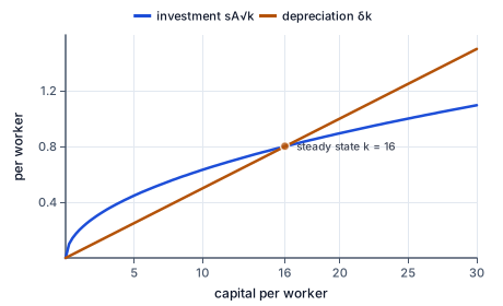
Investment and depreciation per worker against capital per worker, for saving rate 0.2, productivity 1 and depreciation rate 0.05. Investment 0.2√k rises steeply and then flattens; depreciation 0.05k is a straight line. They cross at k = (0.2/0.05)² = 16. Below 16, investment exceeds depreciation and capital grows; above it, capital shrinks.
The figure draws investment and depreciation for one set of parameters: they cross at the positive steady state, and also meet at zero.
A steady state is a capital level that reproduces itself under the transition rule. Set next k equal to k, giving sA square root of k=delta k. For positive k, divide by its square root and solve square root of k=sA/delta. Squaring gives the positive steady state k star=(sA/delta) squared. Every parameter in this expression belongs to the model's stated units and timing.
The division assumes positive capital. At exactly k zero, the square-root production function yields zero output, zero investment and zero depreciation, so zero is also a fixed point. A derivation that divides by square root of k without mentioning this boundary has lost a mathematical solution. The exercises explicitly ask for the positive steady state and start from positive capital.
With A two, s one quarter and delta one eighth, sA/delta is four, so positive steady capital is sixteen. Output there is eight, investment is two and depreciation is two. Consumption is six. These checks verify both the stock equation and the flow resource constraint. A number that solves an algebraic rearrangement should still be substituted into the original economic condition.
For the specified parameter restrictions, the transition function is increasing on positive capital. Below the positive fixed point it produces an increase that stays below that fixed point; above it, it produces a decrease that stays above. Hence positive starting values move toward the positive steady state without crossing it. This conclusion relies on the particular discrete transition and restrictions; a steady-state equation by itself would not prove stability for a different dynamic rule.
Another way: More saving changes a level, not an everlasting growth rate
Raising s increases the positive steady capital and output levels in this model. Starting from the old steady state, the new saving fraction makes investment exceed depreciation, so capital grows during the transition. As capital rises, diminishing returns reduce the extra output generated by another unit, and the system approaches its new steady level. With fixed labor and fixed A, per-worker output growth eventually returns to zero.
This distinction between a level effect and a persistent growth-rate effect matters when reading a policy claim. A permanently higher saving fraction can support permanently higher output without producing a permanently positive growth rate in this particular model. Explaining sustained per-worker growth requires an additional mechanism, such as continuing technological progress, that the fixed-A exercise has not supplied.
The immediate consumption effect also matters. If output is initially fixed, a higher s allocates more of that output to investment and less to current consumption. Future capital may increase, but the change is not a free addition to all dates' consumption. Evaluating the transition requires a criterion for valuing consumption at different dates and across people.
At a steady state, sustainable consumption is f(k)-delta k. For the square-root technology, its derivative is A/(2 square root of k)-delta. The capital level maximizing steady consumption therefore satisfies marginal product equal to depreciation, giving golden-rule capital (A/(2delta)) squared. This is a comparison among steady states. It does not prove that an immediate jump to that capital level is feasible, or that it maximizes discounted utility along the transition.
Another way: Worker growth and technology change the denominator
If the labor force grows, maintaining total capital is not enough to maintain capital per worker. Under a discrete timing convention in which output and depreciation use current workers and next labor is (1+n)L, the transition becomes next k=[(1-delta)k+s f(k)]/(1+n). Dividing only investment by the growth factor would misallocate the surviving old capital among workers.
At a per-worker steady state under that convention, investment must cover both depreciation and capital dilution: s f(k)=(delta+n)k. This exact expression follows from the stated discrete equation. Other definitions, including capital per effective worker when technology also grows, can introduce additional factors. Always derive the denominator from the timing rather than copying a formula from a different convention.
With labor-augmenting technical progress, one can express capital and output per effective worker. A constant value in those units can coexist with rising output per actual worker because each worker's efficiency changes. The meaning of steady state therefore depends on what has been normalized. 'No growth' is ambiguous until the analyst says whether the object is aggregate output, output per worker, or output per effective worker.
The numerical tasks hold labor and A fixed unless an extension explicitly supplies worker growth. This keeps the main calculation transparent and prevents an unexplained growth rate from entering the answer. The extension is a comparison of specified stocks and denominators, not a claim about the demographic or technological path of any real country.
Another way: A production residual is not automatically an explanation
Observed output growth can be decomposed using a production model into contributions from measured inputs and a remaining productivity term. But a residual can include omitted input quality, utilization changes, measurement error and misspecified functional form. Calling it productivity does not identify which invention, institution or organizational change caused it.
Likewise, poorer economies do not necessarily grow faster merely because the marginal product of capital is high in a common production function. The convergence comparison holds other parameters fixed. Different saving behavior, depreciation, population growth, technology, education, institutions or access to finance can imply different steady states or transition mechanisms. Conditional convergence is a model proposition with conditions, not a universal ranking of national growth rates.
A responsible empirical application states what is measured, how capital is constructed, whether depreciation is assumed or estimated, and how labor quality is handled. Historical investment records can support a capital-stock estimate, but the estimate inherits its initial stock and depreciation assumptions. The model is useful because its mechanisms are inspectable; its simplicity is not a substitute for checking whether those mechanisms explain the evidence.
5. A fictional equipment-renewal economy
A planning workshop studies a one-good economy with a fixed number of workers. Output per worker is twice the square root of capital per worker. One quarter of output becomes new capital, one eighth of existing capital depreciates each period, and current capital is four. The units are constructed teaching units, with no foreign borrowing or changes in technology.
Current output is four. Gross investment is one and depreciation is one half, leaving next capital four and one half. Consumption is three. These values reconcile current output's uses and next period's productive stock. Reporting gross investment one as though it were the increase in capital would miss the worn-out half unit that must be replaced.
The positive steady state is sixteen because investment there is two and depreciation is also two. Output is eight and consumption six. The model predicts a transition toward this level from the initial positive stock, rather than an immediate arrival. Its equations do not supply a way to acquire twelve extra units of capital instantly without using resources or changing the institutional assumptions.
A participant proposes raising the saving fraction to one half. At the current output of four, investment would become two and consumption would fall to two. The new positive steady capital would be sixty-four, but the future level does not erase that immediate consumption sacrifice. Comparing the two plans requires a valuation of the full consumption paths. The workshop therefore reports the mechanism and the trade-off, while withholding claims about an actual country's preferred saving policy, feasible financing or long-run technological growth.
6. Check the tempting inference
Positive investment does not guarantee a growing stock. Divide by square root of capital only after separating the zero boundary. Higher saving changes the long-run level in this fixed-technology model, not a permanent per-worker growth rate.
7. Update a capital stock once
State the supplied technology and timing.
y=2sqrt(k); current k 4; s 0.25; delta 0.125
Labor and technology stay fixed.
Calculate current output.
2sqrt(4)=4
The current stock produces this period's output.
Allocate the investment share.
0.25*4=1
The remainder 3 is consumption.
Replace the depreciated portion.
0.125*4=0.5
This part of gross investment maintains existing capacity.
Construct next period's stock.
4-0.5+1=4.5
Net accumulation is only 0.5 despite gross investment 1.
8. Verify a positive steady state
Write the no-change condition.
0.25*2sqrt(k)=0.125k
Gross investment must replace depreciation.
Restrict attention to positive capital.
Divide by sqrt(k)>0
Zero is a separate fixed point and must not be silently discarded.
Solve the resulting linear equation in the root.
sqrt(k)=4; k=16
The square recovers capital units.
Check both flow terms at the candidate.
Investment 2; depreciation 2
The original transition then preserves 16.
Recover sustainable consumption.
Output 8 minus investment 2 equals 6
Steady output still must cover replacement investment.
9. Compare steady consumption without ignoring transition
State a common technology and depreciation.
A 2; delta 0.125
Both candidate saving policies use the same production opportunities.
Find the steady state for saving one quarter.
k 16; output 8; consumption 6
Replacement uses two units of output.
Find the steady state for saving one half.
k 64; output 16; consumption 8
Replacement uses eight units at the larger stock.
Derive the steady-consumption maximum.
MPK=1/sqrt(k)=0.125; k 64
For this technology, marginal extra output equals replacement cost.
Check immediate consumption at initial k 4.
Old consumption 3; new consumption 2
A higher future sustainable level requires an initial sacrifice here.
State the limits of the criterion.
Golden-rule steady consumption is not a discounted transition optimum
Preferences and the entire feasible consumption path are required for that different question.
10. Finish a replacement calculation
Use A 4, s 0.25, delta 0.25 and current k 4.
Output=4sqrt(4)=8
Capital is measured at the start of the period.
Update the stock once.
Next k=3+2=5
One unit depreciates and two are invested.
Your turn: work this step out. Its working is at the end of the packet.
Solve the positive fixed point.
11. Guided practice
Fixed labor and A 2; y=A sqrt(k), saving fraction 0.25, depreciation 0.125, current k 4. Give current y, next k and positive steady k.
Your result
Current output per worker
Next capital per worker
Positive steady capital per worker
12. Guided practice
With fixed labor, y=2sqrt(k), saving 0.5, depreciation 0.25 and current k 9, complete the stock-flow calculation.
Evaluate current production.
output
Use the square root of starting capital.
Carry surviving capital and investment forward.
next
Apply depreciation to the stock and saving to output.
Solve the positive no-change condition.
steady
At a positive steady state, investment exactly replaces depreciation.
13. Guided practice
Fixed labor; y=2sqrt(k), saving 0.25, depreciation 0.125, current k 64. Give current y, next k and positive steady k, retaining any contraction.
Current output per worker: v0. Next capital per worker: v1. Positive steady capital per worker: v2.
14. Practice
Fixed labor; y=4sqrt(k), saving 0.25, depreciation 0.25, current k 9. Give y, next k and positive steady k.
Current output per worker: v0. Next capital per worker: v1. Positive steady capital per worker: v2.
15. Practice
Current total capital 100, labor 10, output 40, saving 0.25 and depreciation 0.1. Next labor is 11; new investment becomes available next period. Produce next total capital, current capital per worker and next capital per worker. Enter the last value to three decimal places.
Next K: v0. Current k: v1. Next k, three decimals: v2.
16. Somewhere new
A fictional equipment economy holds workers and technology fixed. Its y=3sqrt(k), saving is one third, depreciation 0.25 and current k 4. Reconstruct output, next capital and positive steady capital; the fixed saving rule is assumed, not a welfare recommendation.
Current output per worker: v0. Next capital per worker: v1. Positive steady capital per worker: v2.
17. Lesson test
Lesson test: one question per skill, one attempt each, no hints. Your answers are checked when you submit.
18. Test question
A fresh one-good model has constant labor, y=4sqrt(k), saving 0.5, depreciation 0.25 and current k 16. Produce current output, next capital and the positive steady capital level.
Current output per worker: v0. Next capital per worker: v1. Positive steady capital per worker: v2.
19. What you can do now
Reconstruct a fresh case without the worked solution. Explain which assumption would change its conclusion and which result is only an accounting or model condition.
Working for the steps left to you
10. Finish a replacement calculation, step 3
k*=(1/0.25)^2=16
Substitution gives investment 4 and depreciation 4 at that level.