Intertemporal choice

Construct a two-period budget and distinguish feasibility, discounting and borrowing constraints.

Paper packet. Every task here also exists on screen, where it is checked automatically; answers written on paper are not assessed by Nydus. When you are back at a device, enter your answers there.

1. What you will learn

You will construct a two-period budget and distinguish feasibility, discounting and borrowing constraints, showing the calculation and stating the assumptions that make the conclusion valid.

2. Starting point

Use the supplied definitions and units. Separate an accounting identity, a behavioral assumption, and a normative criterion before drawing conclusions.

3. Terms to use precisely

4. Date every resource and every use

Intertemporal choice concerns how resources and consumption are allocated across dates. A unit available today is not automatically interchangeable with a unit available next period. The available saving or borrowing technology determines the rate at which resources can be transferred between those dates. Preferences determine how a person values the resulting consumption patterns. Feasibility and desirability therefore require separate accounts.

Consider a two-period model with incomes y1 and y2, consumption c1 and c2, and a real interest rate r greater than minus one. One unit saved from period one becomes 1+r units in period two. Let s=y1-c1 be saving. Positive s means resources are carried forward; negative s means the person borrows in the first period. With the same rate for borrowing and saving and no other assets, the second-period budget is c2=y2+(1+r)s.

Substituting s=y1-c1 gives c2=y2+(1+r)(y1-c1). Rearranging yields c1+c2/(1+r)=y1+y2/(1+r). Both sides are now measured in period-one consumption units. The right side is the present value of the two income flows under this transfer technology. It is a wealth measure within the model, not the amount of cash available immediately without access to borrowing.

The accounting equality assumes that all available lifetime resources are used by the end and that there is no terminal bequest or unmodeled debt. If disposal or leftover assets are allowed, the feasible set can instead use an inequality. Stating this terminal condition prevents the equation from silently treating an unpaid final debt as free resources or excluding a desired bequest without acknowledgment.

Term	What it means
Present value	A future resource converted into current units at the specified transfer rate.
Saving	Current income minus current consumption in the two-period account.
Borrowing constraint	A limit on transferring future resources into the present through debt.
Preference discount factor	The weight on future utility, distinct from the market interest rate.
Euler condition	An interior marginal-utility trade-off linking consumption across dates.

Another way: Present value is a conversion rule, not a preference statement

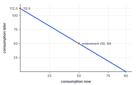
Future consumption against current consumption for a person earning 50 now and 50 later, who can save or borrow at 25 percent. Each unit consumed now costs 1.25 units later, so the budget line has slope −1.25. It passes through the endowment point (50, 50), reaches 112.5 if everything is saved and 90 if everything is borrowed against.

The figure draws a two-period budget at a 25 percent rate: a line of slope −1.25 through the endowment.

Discounting a future resource by 1+r converts it into its period-one equivalent at the available market transfer rate. For example, with r one quarter, twenty-five future units have present value twenty. Saving twenty now produces twenty-five later. This equivalence follows from the specified technology or contract, not from a claim that the person emotionally values future consumption less.

A preference discount factor is a different object. A utility function might be U(c1,c2)=u(c1)+beta u(c2), where beta weights future utility. The market interest rate r belongs to the budget; beta belongs to preferences. A person can care greatly about the future and still face an expensive borrowing opportunity, or prefer current consumption while facing a high return to saving. Conflating the two erases the economic trade-off.

The budget slope in a graph with c1 on the horizontal axis and c2 on the vertical axis is negative (1+r). Increasing current consumption by one unit reduces feasible future consumption by 1+r units, holding incomes and the transfer rule fixed. The intercepts follow from setting each consumption quantity to zero, subject to any additional limits. A borrowing restriction can remove part of that line from the feasible set.

Nominal amounts need a separate price adjustment if the consumption unit changes in purchasing power across dates. This lesson uses a stated real rate and a common consumption unit, so inflation is not part of its arithmetic. The later expectations lesson distinguishes nominal returns, expected inflation and realized purchasing power. Do not mix a nominal income flow with a real rate without making the units consistent.

Another way: A borrowing constraint changes feasibility

Suppose a person is not allowed to borrow. Then saving must satisfy s at least zero, which means c1 cannot exceed y1. Future income still contributes to lifetime resources, but it cannot be moved backward to finance current consumption through the prohibited transaction. A present-value budget alone would falsely describe some unavailable plans as feasible unless this additional inequality were included.

For y1 twenty, y2 forty and r zero, lifetime resources total sixty. The unrestricted plan c1 thirty and c2 thirty satisfies the lifetime budget, but it requires borrowing ten in the first period. Under the no-borrowing condition, that plan is infeasible. The endowment plan c1 twenty and c2 forty is feasible, as are plans with lower current consumption and positive saving.

A limited borrowing rule can be written s at least minus B, where B is the maximum permitted loan principal in period-one units. This gives c1 at most y1+B. Nonnegative future consumption also requires c1 at most y1+y2/(1+r), so the overall maximum is the smaller of that bound and y1+B. A debt-service limit expressed in period-two units would instead need conversion by 1+r. Naming which date the limit refers to avoids a common units error when applying the constraint.

Collateral, verification, default risk and institutions can affect borrowing opportunities in real settings. The simplified limit is a constraint supplied to the exercise, not an explanation of every credit restriction. The information lesson showed why an inability to observe type or effort can matter for lending terms. Here the purpose is to account correctly for a given limit before deriving or judging a consumption plan.

Another way: Optimal smoothing depends on preferences and constraints

For an interior optimum with differentiable utility u(c1)+beta u(c2), the first-order condition is u'(c1)=beta(1+r)u'(c2). Moving a small resource unit from current consumption to saving gives up marginal utility now and gains 1+r future units weighted by beta. Equality holds only when the optimum is interior and the transfer is feasible in both directions.

With logarithmic utility and positive consumption, marginal utility is one divided by consumption. The condition becomes c2=beta(1+r)c1. If beta is one, optimal present spending on consumption is equally divided between dates: c1 equals half of present-value income and c2 equals (1+r)c1. Equal present-value spending is not necessarily equal physical consumption when the interest rate is nonzero.

If the unconstrained solution requires borrowing beyond the allowed limit, the optimum can lie at that boundary. For logarithmic utility with y1 twenty, y2 forty, r zero and beta one, the unrestricted solution is thirty in each period. With borrowing prohibited, the best feasible current consumption is twenty and future consumption forty. The marginal utility equality fails at that constrained optimum because the desired transfer toward the present is unavailable.

The word smoothing therefore does not prescribe identical consumption in every period. The shape of utility, the preference weight, expected income, the rate and constraints all matter. Uncertainty can also produce precautionary saving under additional conditions. This deterministic two-period model provides a transparent starting point; it should not be described as a complete explanation of household financial behavior.

Another way: An interest-rate change has more than one channel

A higher real rate makes current consumption more expensive in terms of forgone future consumption, creating a substitution incentive toward the future. It also changes the value of a person's existing asset or debt position and the attainable budget. A saver and a borrower can experience different income effects. Consequently, one cannot infer the total saving response from the substitution channel alone.

The budget line always passes through the endowment point (y1,y2) in this simple model. Consuming each income when received requires no transfer, so changing the rate does not alter that particular feasible allocation. The line rotates around the endowment point. On the saving side a higher rate delivers more future consumption for the same current sacrifice; on the borrowing side it requires more future repayment for the same current advance.

If borrowing and saving rates differ, the feasible boundary can have a kink at the endowment point. A single straight-line formula is no longer valid over both sides. Fees, default possibilities, taxes and uncertain returns can introduce further differences. The exercise's assumption of one known common rate is therefore substantive rather than a harmless notation choice.

Comparative statics should specify what remains fixed when the rate changes. If a macroeconomic event simultaneously alters employment, expected income and asset values, an observed saving change cannot be attributed solely to the rate without further evidence. The model identifies possible channels; empirical work must establish which channels moved and how strongly in the setting being studied.

Another way: Check the two dated budgets as well as the consolidated one

A useful audit computes saving from the first-period account and then reconstructs second-period consumption. If c1 is thirty, y1 forty and r one fifth, saving is ten and carries twelve units forward. With y2 twenty-four, c2 is thirty-six. The present-value equation then gives thirty plus thirty-six divided by 1.2, equal to sixty, matching forty plus twenty-four divided by 1.2. This second calculation checks arithmetic and units independently. It does not replace the separate check for a borrowing limit, nonnegative consumption and the terminal condition. A plan can balance the lifetime account while violating an institutional constraint, just as an algebraic optimum can lie outside a feasible set.

Another way: Income timing matters when credit is limited

Two income sequences can have the same present value and different constrained consumption opportunities. Moving income from the first period into the second leaves unrestricted wealth unchanged if the future increase exactly includes the transfer return. Under a binding borrowing limit, however, that change can reduce the largest feasible current consumption. This is a concrete reason liquidity and wealth are different concepts. It also explains why an income payment's timing can affect behavior even when its present value is unchanged; the conclusion follows from a constraint rather than from an assumption that people ignore the future.

5. A fictional two-season workshop budget

A workshop's owner plans personal consumption over two teaching seasons using a deliberately simplified real-resource account. Income is forty consumption units in the first season and twenty-four in the second. The known real transfer rate is twenty percent, the same for saving and borrowing, and there is no initial wealth, terminal bequest or unpaid final debt. The owner proposes consuming thirty units in the first season.

Saving is forty minus thirty, or ten units. Those units deliver twelve in the second season, so second-season consumption can be thirty-six. Present-value consumption is thirty plus thirty-six divided by 1.2, equal to sixty. Present-value income is forty plus twenty-four divided by 1.2, also sixty. The two dated budgets and the consolidated budget agree.

A different proposal calls for first-season consumption fifty. It requires borrowing ten and repaying twelve later, leaving twelve units for second-season consumption. That plan balances the unrestricted lifetime account. If the borrowing limit is only five first-season units, however, the proposal is infeasible even though lifetime resources are sufficient. The largest permitted current consumption would then be forty-five.

The exercise deliberately stops short of advising which plan the owner should select. A utility function, risk attitudes, uncertain expenses and real borrowing terms would be needed for that judgment. Its immediate purpose is to separate resource conversion from preferences and to show why a future income stream does not remove a current borrowing constraint. Every stated quantity uses the same real consumption unit, so inflation has not been silently mixed into the calculation.

6. Check the tempting inference

A market discount rate converts resources; a preference weight values utility. A present-value budget does not override a borrowing limit. Apply the gross factor 1+r, distinguish loan principal from repayment, and state whether rates are real or nominal.

7. Carry saving forward and check both accounts

8. Detect a borrowing-limit violation

9. Derive an interior log-utility allocation

10. Complete a borrowing account

11. Guided practice

Real two-period incomes are 40,24; rate 0.2; proposed current consumption 30. Loan principal cannot exceed 5 current units. Produce saving, implied future consumption and maximum permitted current consumption. No terminal asset or debt remains.

12. Guided practice

Real incomes are 30,24, rate 0.2 and proposed current consumption 25. Borrowing is prohibited. Complete saving, future consumption and maximum current consumption under the constraint.

13. Guided practice

Real incomes 24,40; common borrowing/saving rate 0.25; proposed c1=28; loan-principal limit 3. Produce signed saving, implied unrestricted c2 and the separate maximum feasible c1.

	Your result
Saving, negative if borrowing
Implied second-period consumption
Maximum feasible first-period consumption