Back to the on-screen lesson ·
Construct AD schedules and distinguish movements, shifts, mechanisms, and missing equilibrium information.
Paper packet. Every task here also exists on screen, where it is checked automatically; answers written on paper are not assessed by Nydus. When you are back at a device, enter your answers there.
Plot declared aggregate-demand points, compare fixed-price spending shifts, and construct conditional transmission arguments while identifying monetary and international assumptions.
You know that domestic expenditure is C + I + G + X - M and that actual output can differ from potential. Aggregate demand introduces a behavioral model connecting planned spending to the overall price level. The accounting identity alone does not supply that relationship; the model must state how spending responds and what is held fixed.
| Term | What it means |
|---|---|
| Aggregate demand | Planned expenditure on domestic final output at each price level under stated conditions. |
| Movement along AD | A change in quantity of aggregate output demanded caused by a change in the price level, with other determinants held fixed. |
| Shift of AD | A change in planned domestic spending at a given price level due to another determinant. |
| Real balances | The purchasing power of a nominal money balance after adjustment for the price level. |
| Autonomous spending | Spending specified as independent of current income within the particular model. |
A conventional aggregate-demand diagram places real output on the horizontal axis and an aggregate price-level index on the vertical axis. A point on the curve describes planned domestic expenditure at that price level, given the model's other conditions. The vertical axis is not the price of one product, and the horizontal axis is not the quantity of that product. Confusing these axes imports a single-market story into an economy-wide model.
For a fictional schedule, let planned real spending Y equal 200 minus the price index P over the displayed positive range. At P equal to eighty, Y is 120. At P equal to one hundred, Y is one hundred. At P equal to 120, Y is eighty. When plotting these observations, the coordinates are (120,80), (100,100), and (80,120), because real output comes first. The algebra's order of presentation does not reverse the graph's declared axes.
This straight schedule is supplied for transparent arithmetic, not estimated from an actual economy. It captures a negative relationship under the stated conditions. The economic explanation of that relationship requires mechanisms linking the aggregate price level to consumption, investment, and net exports. Those mechanisms depend on monetary conditions, international arrangements, and other assumptions that must accompany the curve.
Another way: steps
Identify whether the changing variable is the price level or another spending determinant. For a price-level change, read a new point on the existing schedule. For another determinant, construct a shifted schedule at the same price levels before comparing outcomes.
One channel is a real-balance or wealth effect. If a household holds a fixed nominal money balance, a lower price level raises the basket quantity that balance can purchase. Under an assumed positive consumption response, planned consumption rises. This mechanism concerns the purchasing power of nominal assets. It does not imply that every household becomes wealthier in net terms, because nominal liabilities and distributional positions also matter.
A second introductory channel works through interest rates. In a model holding the nominal money supply fixed, a lower price level reduces the nominal balances needed for a given volume of transactions. Under the specified money-market adjustment, interest rates fall, which can raise interest-sensitive investment and consumption. Each link is conditional. If a central bank instead adjusts its instruments to maintain a particular interest-rate target, the simple fixed-money-supply story is not automatically the operating description.
A third channel concerns relative prices and net exports. Holding foreign prices and nominal exchange rates fixed, a lower domestic price level makes domestic products relatively cheaper to foreign buyers and imported products relatively dearer to domestic buyers. Under appropriate quantity responses, exports rise and imports fall, increasing net exports. The fixed exchange-rate and foreign-price conditions are part of this mechanism. Exchange-rate movement or weak trade responses can alter the result.
These channels are not the claim that consumers substitute one domestic product for another when its relative price falls. An aggregate price-level change concerns a broad set of domestic prices. Nor does a downward AD curve prove that falling prices always restore a depressed economy quickly. Debt burdens, expectations, banking conditions, and policy responses can complicate the adjustment. The curve represents a particular relationship under held-fixed conditions, not a universal policy instruction.
To explain a movement along the curve, identify which of these model channels is assumed to operate and preserve the other determinants. If the exercise simply supplies an algebraic schedule, the numerical points follow from that schedule. The explanatory text should still distinguish the supplied relationship from a claim that the coefficient or mechanism has been measured in a real country.
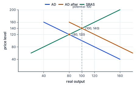
The figure shows a shift: at every price level, planned spending rises, so the whole curve moves right.
Suppose firms become more optimistic about future sales and increase planned investment at every displayed price level. In the fictional schedule, AD changes from Y = 200 - P to Y = 220 - P. At P equal to one hundred, planned spending rises from one hundred to 120. The horizontal shift is twenty output units at every displayed price level. The event changes a nonprice determinant, so it shifts AD rather than causing movement along the original curve.
Government purchases can also shift planned expenditure, other things equal. A tax change can affect disposable income and consumption, with a response depending on the assumed spending propensity. A change in foreign demand can affect exports. Changes in credit availability, household expectations, or financial wealth can influence private expenditure. A list of possible shifters is useful only when connected to a specific component and mechanism rather than memorized as automatic directional slogans.
For example, a fall in a stock-market index does not establish the exact change in consumption without a model linking that wealth change to spending. A rise in government purchases does not establish a particular net AD shift if taxes, interest rates, or other components change simultaneously. Introductory items hold those other influences fixed or provide their changes explicitly. When they do not, the conclusion may be underdetermined.
Distinguish a change in investment spending from buying an existing financial asset. Purchasing a newly produced machine enters investment in the expenditure account. Trading an existing share does not directly purchase new output, although asset prices and financing conditions can affect later spending decisions. Likewise, a government transfer affects demand through recipients' behavior rather than entering G as a direct purchase. The accounting distinctions from the circular-flow lesson remain essential.
A curve can shift left when planned domestic spending falls at each price level. In the example, changing the intercept from 200 to 180 reduces Y by twenty at a fixed P. It does not by itself specify the new equilibrium price or actual output. Those outcomes require aggregate supply and an adjustment mechanism, which the next lessons introduce. AD is one relationship in a model, not a complete prediction on its own.
Two events can push aggregate demand in opposite directions. Suppose a fictional fiscal expansion raises planned domestic expenditure by thirty units at each price level, while a fall in private investment lowers it by twenty. If the model says those effects are additive and no other component responds, the net horizontal shift is ten units to the right. The calculation follows from the supplied magnitudes, not from deciding that fiscal changes always dominate private changes.
If only the directions are given, the net direction may be unknown. An export increase and a consumption decrease cannot be combined into a definite AD shift without knowing their relative sizes or additional restrictions. A correct answer can state the competing mechanisms and the missing magnitude. Economic reasoning does not always produce an increase-or-decrease verdict from qualitative information alone.
The distinction between movement and shift can also coexist in one comparison. If AD shifts from Y = 200 - P to Y = 220 - P while the observed price level rises from one hundred to 110, planned spending changes from one hundred to 110. The twenty-unit rightward shift and the ten-unit reduction associated with the higher price level yield a net ten-unit increase. Reporting only the shift or only the price movement would miss part of the stated change.
Decomposing changes requires a declared order or a model in which the components are separable. Our linear additive example has a constant slope and a parallel shift, so the decomposition is transparent. With nonlinear curves or interactions, the measured contribution of each change can depend on the comparison path. That is a reason to name the model's form and avoid treating every graph shift as a fixed numerical effect.
Finally separate planned demand from realized output. Firms may respond to a spending change through inventories, production, prices, or a combination, depending on capacity and adjustment conditions. The identity between realized output and realized expenditure remains valid through inventory accounting, but that does not mean a planned-spending schedule is automatically fulfilled at every point. An equilibrium model identifies the conditions under which the relevant plans are mutually consistent.
This careful interpretation makes graphs useful for comparing assumptions. A fixed-money model and an interest-rate-target model can transmit a price-level change differently. A closed-economy model omits the net-export channel. The learner should be able to identify which link changes when an assumption changes, rather than treating disagreement about mechanisms as a failure of arithmetic.
A fictional economy's initial AD schedule is Y = 200 - P, where Y is real output in base-year dollars and P is a price index. A case specifies that new government purchases add thirty units to planned expenditure at every price level, while firms simultaneously reduce planned investment by twenty units. Taxes, monetary conditions, foreign spending, and every other determinant remain fixed. The model also states that the two shifts combine additively.
The new schedule is Y = 210 - P. At an unchanged price index of one hundred, planned domestic expenditure rises from one hundred to 110. A report claiming that AD rose by thirty ignores the simultaneous private-investment change. A report claiming that actual output must rise by ten goes beyond the information supplied, because aggregate supply and the equilibrium price adjustment have not yet been specified.
Suppose the case additionally observes a later price index of 105. The new schedule gives planned expenditure of 105. Relative to the original point (100,100), the final point is (105,105). The rightward schedule shift raises demand at a fixed price, while the higher price moves along the new schedule in the opposite direction. The net change in the demanded quantity is five in this combined comparison.
The useful conclusion states the schedule change, the fixed-price comparison, and the actual point comparison separately. It also names the additive and held-fixed assumptions. This is a complete model calculation without becoming a recommendation for government spending or a forecast about a real economy.
The AD vertical axis is the aggregate price level, not the price of one good. A price-level change moves along a given AD relationship; a nonprice spending determinant shifts it. A shift alone does not determine actual equilibrium output. Opposing shifts cannot be ranked without magnitudes. A monetary mechanism assuming a fixed money supply must not silently be treated as an interest-rate-target regime.
State the supplied relationship and axis order.
Y = 200 - P; horizontal Y, vertical P.
The graph's coordinate order is output followed by the price index.
Evaluate the low-price observation.
P=80 gives Y=120.
Other spending determinants remain fixed in this calculation.
Evaluate the middle observation.
P=100 gives Y=100.
The same schedule supplies a second planned-spending quantity.
Evaluate the high-price observation.
P=120 gives Y=80.
The supplied slope gives lower planned spending at a higher price level.
Write the graph coordinates.
(120,80), (100,100), and (80,120).
Placing the price index first would reverse the declared axes.
Record the original relationship.
Y = 200 - P.
This is the baseline planned-spending schedule.
Record the investment-driven new relationship.
Y = 220 - P.
The nonprice change adds twenty units at every price level.
Compare at the same price index.
At P=100, Y rises from 100 to 120.
Holding price fixed isolates the shift.
Then evaluate a higher price on the new schedule.
At P=110, new Y=110.
This is movement along the shifted relationship.
State the combined change.
Original Y=100; final Y=110; net increase ten.
The twenty-unit shift and ten-unit price response act in opposite directions.
Identify the initial intercept and slope.
Initial Y = 200 - P.
The model supplies a linear spending relationship.
Enter the public-purchase shift.
Add thirty to planned expenditure at each P.
This event changes G rather than the price level.
Enter the private-investment shift.
Subtract twenty at each P.
The case explicitly supplies the simultaneous offset.
Construct the resulting schedule.
New Y = 210 - P.
Additivity and unchanged remaining determinants make the net shift ten.
Evaluate the observed later price.
At P=105, Y=105.
The price response moves along the new curve after the shift.
State the remaining information requirement.
An equilibrium prediction still needs aggregate supply or a specified realized price.
A demand relationship alone does not determine both price and output.
Record both supplied schedules.
Initial Y=180-P; new Y=160-P.
The intercept falls while the slope remains unchanged.
Evaluate them at price index eighty.
Initial Y=100; new Y=80.
Holding P fixed isolates the change in a nonprice determinant.
Describe the scope of the result.
A fictional model specifies Y=180-P for planned real domestic expenditure in base-year dollars. Complete Y for the three price-index values; all other determinants are fixed.
| Y base-year dollars | |
|---|---|
| P=60 | |
| P=80 | |
| P=100 |
A fictional model begins at Y=250-P. Investment rises by thirty at every price index while consumption falls by eight. Effects are additive; the price index used for comparison is one hundred. Complete the shift and the new point.
Combine the two spending changes.
Net intercept change = shift.
The changes enter with opposite signs.
Construct the new intercept.
New intercept = intercept.
The original relationship retains its slope under the stated parallel shift.
Evaluate planned spending at the supplied price.
New Y = quantity.
Subtract the comparison price index from the new intercept.
Plot the fictional AD points implied by Y=160-P at P=40,60,80. Horizontal axis is real output Y in base-year dollars; vertical axis is price index P.
Plot your answer on the grid:
A fictional initial schedule is Y=240-P. A stated confidence change adds twenty to investment demand at every P, with no offsets. Complete initial and new Y at the listed price indexes.
| Initial Y | New Y | |
|---|---|---|
| P=100 | ||
| P=120 |
Construct the stated fixed-nominal-money mechanism for a lower price level. Assume lower transaction demand for nominal balances reduces interest rates and investment responds inversely to rates. Do not assume this describes every monetary regime.
This task has no paper form; do it on a device.
A fictional island has Y=300-P. Higher foreign demand adds forty to exports at every P, while a separate household-spending reduction subtracts ten. The effects are additive and all other determinants stay fixed. At P=120, compute initial Y, net shift, and new Y.
| Real output units | |
|---|---|
| Initial Y | |
| Net horizontal shift | |
| New Y |
Lesson test: one question per skill, one attempt each, no hints. Your answers are checked when you submit.
A fictional economy initially has Y=220-P and P=100. A stipulated fiscal change adds twenty-five to planned spending, while another event reduces investment by five; effects are additive. The later observed P is 110. Compute the net shift, new intercept, original Y, and later Y.
| Value | |
|---|---|
| Net shift | |
| New intercept | |
| Original Y | |
| Later Y |
You can distinguish a price-level movement from a nonprice demand shift and combine supplied offsets. Next, add short-run and long-run supply relationships before solving an aggregate equilibrium.
13. A leftward demand shift at a fixed price, step 3
Demand shifts twenty units left; equilibrium output is not yet determined.
A supply relationship is required to close the aggregate model.