Back to the on-screen lesson ·
Compare price movements, cost shocks, productivity changes, and long-run capacity.
Paper packet. Every task here also exists on screen, where it is checked automatically; answers written on paper are not assessed by Nydus. When you are back at a device, enter your answers there.
Plot declared SRAS points, construct fixed-price supply comparisons, and distinguish temporary cost shifts from changes in potential while explaining the assumptions behind short-run and long-run adjustment.
Aggregate demand gives planned spending at each price level. An equilibrium also requires a relationship describing firms' aggregate production responses. The short-run supply relationship will hold some costs and expectations fixed, while the long-run capacity benchmark allows a different set of adjustments.
| Term | What it means |
|---|---|
| Short-run aggregate supply | The relationship between price level and aggregate production under stated temporarily fixed input prices or expectations. |
| Sticky nominal wage | A wage in dollars that does not adjust immediately to every change in prices or conditions. |
| Long-run aggregate supply | The sustainable output benchmark determined by real productive conditions in the introductory model. |
| Supply shock | A change in costs or productive conditions that shifts aggregate supply. |
| Expected price level | The price level anticipated when contracts or production decisions are set. |
A common introductory SRAS model assumes some nominal wages or other input costs are temporarily fixed by contracts or adjustment frictions. If selling prices rise while those costs remain unchanged, producing additional output can become more profitable. Firms expand production along an upward-sloping short-run relationship. This is a conditional mechanism, not a claim that firms can increase physical capacity indefinitely whenever prices rise.
For a fictional schedule, suppose the price index satisfies P = 40 + 0.5Y, where Y is real output in base-year dollars. At Y equal to eighty, P is eighty; at Y equal to 120, P is one hundred; at Y equal to 160, P is 120. The graph has real output on the horizontal axis and the price index vertically, so the three points are (80,80), (120,100), and (160,120).
Long-run aggregate supply is drawn vertically at potential output in the simple model. Once wages, input prices, and expectations have adjusted, a higher general price level alone does not permanently increase the economy's real productive resources. If potential output is 120, LRAS is the vertical line Y = 120. The vertical line does not say actual production can never differ from 120 for a time; it identifies the longer-run benchmark under the supplied conditions.
Another way: steps
Identify the time horizon and the costs or expectations held fixed. Use a price-level change to move along the existing short-run schedule. Use a cost or productivity change to shift supply. Track potential separately when the event changes sustainable capacity.
The sticky-wage explanation distinguishes nominal and real labor cost. If a worker's nominal wage is fixed at twenty dollars while the output-price index rises, the wage buys less output and the producer's labor cost relative to its selling price falls. Under the model's labor-demand and production assumptions, the firm may hire more hours and expand output. This conclusion depends on input-cost rigidity and available productive responses, not on a general rule that inflation creates resources.
Other introductory explanations use imperfect information or temporarily sticky product prices. A producer may initially interpret a rise in its selling price as an improvement relative to other prices, or some firms may adjust prices more slowly than others. These are alternative mechanisms for short-run nonneutrality. A lesson should not mix them casually as though each requires exactly the same assumptions. The assessed numerical schedule simply states its relationship, while the mechanism question names the relevant rigidity.
The slope of SRAS can vary with capacity use and adjustment conditions. A relatively flat relationship represents a setting in which output can respond substantially with limited price adjustment over the relevant range. A steeper relationship represents a setting where additional spending mainly affects prices. The shape is a model assumption or an empirical question, not a universal constant. Our straight-line examples are local teaching relationships with explicitly limited ranges.
Short run does not mean one fixed number of months for every economy. It refers to which prices, contracts, and expectations have not yet adjusted in the model. A rapidly renegotiated contract can change the relevant horizon, while other rigidities persist longer. Likewise, long run is not a promise that adjustment completes on a known calendar date. It is a comparison allowing the adjustments that define the model's longer-run equilibrium.
A movement along SRAS caused by a higher price level differs from an outward shift caused by better technology. In the first, the cost and productivity conditions are fixed. In the second, firms can produce more at a given price level because the underlying production or cost relationship changes. Graphs help only when the author identifies which variable changed and which remained fixed.
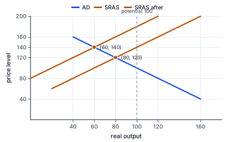
The figure shows a cost shock: the short-run supply curve moves up, raising the price level and lowering output.
Suppose imported energy becomes more expensive in a fictional economy, raising production costs at each output level. Holding other factors fixed, the SRAS schedule can shift upward or leftward: a higher price level is required to support the same output, or less output is supplied at the same price level. If P = 40 + 0.5Y becomes P = 60 + 0.5Y, the vertical shift is twenty index points. At P equal to one hundred, supplied output falls from 120 to eighty.
That cost shock need not permanently reduce potential output. If it is temporary and does not damage resources or technology, the long-run benchmark may remain unchanged in the stipulated case. A persistent energy constraint or destruction of productive equipment could instead reduce potential. The event's duration and effect on real capacity determine whether LRAS shifts too. Do not automatically shift both curves whenever the word supply appears.
A productivity improvement can reduce unit costs and expand sustainable productive capacity. Under a stated scenario, SRAS shifts down or right and LRAS shifts right. For example, a process improvement may change SRAS from P = 40 + 0.5Y to P = 30 + 0.5Y while raising potential from 120 to 140. The two changes need not have the same numerical size or follow one fixed formula. The model must supply the relationships being compared.
An increase in expected prices can shift SRAS upward if workers negotiate higher nominal wages or firms revise input contracts in anticipation. At each actual price level, those higher nominal costs reduce the incentive to produce relative to the previous schedule. This expectations channel explains why a short-run response can change over time even when current aggregate demand is unchanged. It also connects to later analysis of inflation expectations and the Phillips curve.
Supply-shift labels describe conditional relationships, not policy judgments. A nominal wage increase can have different aggregate consequences depending on productivity, demand, distribution, and the degree of wage-setting flexibility. The simplified cost-shift exercise isolates one channel with other factors fixed. It should not be used to conclude that wages ought to fall or that any particular real labor-market institution is undesirable.
In a basic AD–AS account, output above potential puts upward pressure on wages or expected prices over time. SRAS shifts upward until the economy returns to potential at a higher price level, if aggregate demand and potential remain fixed. Output below potential can create downward cost pressure and a gradual rightward SRAS shift. These mechanisms describe a possible adjustment path under flexible-enough eventual costs, not an instantaneous return to equilibrium.
Several assumptions are doing work. Potential must remain unchanged; spending must not shift again; financial distress or permanent damage must not alter productive capacity; and costs must adjust in the specified direction. If expectations change quickly, if nominal wages resist downward adjustment, or if a recession reduces investment and labor-market attachment, the path can differ. Identifying these assumptions is more informative than saying that the economy always fixes itself or never adjusts at all.
The long-run vertical curve also distinguishes a price-level change from economic growth. A rise in aggregate demand can produce a higher long-run price level with unchanged potential in this model. Sustained growth of real output requires changes in productive resources, technology, or institutional conditions that expand capacity. The growth lesson will examine these mechanisms directly rather than treating an upward price movement as increased long-run wealth.
Money neutrality in a particular long-run model is likewise a conditional proposition. It states that changing a nominal quantity does not permanently alter real output once the model's adjustments have occurred, holding relevant real determinants fixed. It does not mean monetary disturbances have no short-run consequences, that financial institutions are irrelevant, or that every historical episode has the same adjustment path. Keep the proposition's horizon and assumptions attached to it.
When comparing two models, ask where they disagree. One might assume rapid expectation adjustment and another slow nominal-wage adjustment. Both can solve their own equations correctly and produce different short-run output responses. The substantive question is which assumptions fit the case, supported by evidence. Machine-graded tasks can assess the conditional predictions and the differing assumptions without grading agreement with a policy position.
A fictional economy begins with SRAS given by P = 40 + 0.5Y and potential output of 120 base-year dollars. A temporary shipping disruption raises input costs so that SRAS becomes P = 60 + 0.5Y. The case explicitly states that equipment, labor skills, and sustainable productive capacity are unchanged. At a price index of one hundred, the initial supplied quantity is 120 and the new supplied quantity is eighty.
The right comparison holds the price index fixed while changing the cost schedule. The forty-unit reduction in supplied output at that price is a short-run shift, not movement along the original curve. LRAS remains at Y = 120 under the stated no-capacity-loss assumption. The new equilibrium cannot be computed until aggregate demand is supplied, because price may change as both sides adjust.
Now compare a different case in which a storm destroys productive equipment permanently. Suppose the case supplies potential output of one hundred afterward, together with its own new SRAS equation. LRAS shifts left in that second model because sustainable capacity has changed. The two events may both be described informally as supply problems, but their long-run implications differ because the resource assumptions differ.
A careful analyst records the temporary cost equation, the potential benchmark, and the missing demand relationship separately. The analyst does not infer a monetary or fiscal recommendation from the curve shift alone. Decisions would also require the expected duration, distribution of losses, available tools, and consequences of alternative responses. The diagram supports conditional reasoning rather than replacing those questions.
A higher general price level moves along a given SRAS relationship when costs and expectations are fixed. A cost shock shifts that relationship. A temporary cost change need not alter potential, while durable resource loss can. Vertical LRAS does not forbid temporary deviations from potential. Long-run adjustment requires assumptions about costs, expectations, and unchanged real capacity.
State the relationship and units.
P=40+0.5Y, with Y in base-year dollars.
The equation applies under fixed short-run cost conditions.
Evaluate the first output level.
Y=80 gives P=80.
The price index follows the stated positive slope.
Evaluate the central output level.
Y=120 gives P=100.
This point also coincides with the supplied potential in the example.
Evaluate the higher output level.
Y=160 gives P=120.
Output above potential is possible temporarily under the model.
Write the coordinate pairs.
(80,80), (120,100), (160,120).
Real output is horizontal and the price index is vertical.
Record the original schedule.
P=40+0.5Y.
This is the benchmark under the initial input costs.
Record the shifted schedule.
P=60+0.5Y.
The temporary cost increase raises the intercept by twenty.
Solve the original quantity at P=100.
100-40=0.5Y, so Y=120.
Holding price fixed isolates the schedule comparison.
Solve the new quantity at the same price.
100-60=0.5Y, so Y=80.
Higher costs reduce quantity supplied at the unchanged price level.
State the potential-output condition.
Potential remains 120 if sustainable capacity is explicitly unchanged.
A short-run cost shift does not automatically imply a long-run capacity loss.
Fix the common starting capacity.
Potential output 120 base-year dollars.
Both cases begin from the same long-run benchmark.
Identify the first event's scope.
Temporary freight costs rise; productive resources remain intact.
The case changes current costs without changing sustainable capacity.
Represent the first event.
SRAS shifts upward; LRAS remains at Y=120.
The distinction follows the explicitly limited cost shock.
Identify the second event's scope.
A different storm permanently destroys productive equipment.
This event changes a real determinant of sustainable output.
Represent the supplied second benchmark.
If new potential is 100, LRAS shifts to Y=100.
The long-run shift records the stipulated capacity loss.
State what both cases still require.
Aggregate demand is needed to solve the equilibrium price and output.
A supply relationship alone does not determine the intersection.
Record the initial and improved supply equations.
Initial P=50+0.5Y; improved P=40+0.5Y.
The innovation reduces costs at every displayed output level.
Compare output at price index one hundred.
Initial Y=100; improved Y=120.
The fixed-price comparison shows a rightward short-run supply shift.
Track the separately supplied potential change.
A fictional short-run model holds nominal input costs fixed and specifies P=20+0.5Y. Complete the price index at each real-output value in base-year dollars.
| Price index P | |
|---|---|
| Y=80 | |
| Y=120 | |
| Y=160 |
A fictional SRAS equation is P=35+0.5Y. Evaluate it at Y=90. A cost shock then raises its intercept by fifteen while keeping Y fixed for comparison. Complete the calculations.
Evaluate the original price index.
Original P=initial.
Substitute the specified real output into the initial relationship.
Update the cost intercept.
New intercept=intercept.
The shock adds its stated amount to the intercept rather than to output.
Evaluate the shifted equation at the same output.
New P=new.
The fixed-output comparison isolates the vertical supply shift.
Plot the fictional SRAS observations implied by P=30+0.5Y at Y=40,80,120. Real output Y in base-year dollars is horizontal; price index P is vertical.
Plot your answer on the grid:
A fictional temporary input-cost shock changes SRAS from P=30+0.5Y to P=50+0.5Y. Potential remains 140 base-year dollars. At P=100, compute initial supplied output, new supplied output, and the change in potential.
| Base-year dollars | |
|---|---|
| Initial supplied output | |
| New supplied output | |
| Potential-output change |
Construct the stipulated short-run mechanism. Nominal wages are fixed, selling prices rise, and firms can expand hours when labor cost relative to output price falls.
This task has no paper form; do it on a device.
A fictional island's process improvement changes SRAS from P=60+0.5Y to P=40+0.5Y and separately raises potential from 100 to 140 base-year dollars. At price index one hundred, compute old supplied output, new supplied output, and new potential.
| Base-year dollars | |
|---|---|
| Old supplied output | |
| New supplied output | |
| New potential |
Lesson test: one question per skill, one attempt each, no hints. Your answers are checked when you submit.
A fictional economy has initial SRAS P=20+0.5Y and potential 160 base-year dollars. A temporary cost shock raises the SRAS intercept to forty, with potential explicitly unchanged. At P=100, compute initial supplied output, new supplied output, the horizontal change at that price, and potential after the shock.
| Base-year dollars | |
|---|---|
| Initial supplied Y | |
| New supplied Y | |
| Change in supplied Y | |
| Potential after shock |
You can identify which supply relationship changes and why, without treating a temporary shock as permanent capacity loss. Next, combine demand and supply to solve equilibrium and compare shocks.
13. A specified productivity improvement, step 3
If potential rises from 100 to 120, LRAS also shifts right.
The long-run result depends on the stated productivity effect on sustainable capacity.