Back to the on-screen lesson ·
Distinguish actual growth, cycle turning points, estimated capacity, and evidence from indicators.
Paper packet. Every task here also exists on screen, where it is checked automatically; answers written on paper are not assessed by Nydus. When you are back at a device, enter your answers there.
Plot supplied output paths, compute output gaps and growth with appropriate denominators, and compare capacity revisions without treating cycle patterns or leading indicators as guaranteed forecasts.
You can measure real production and classify labor-market status. Now compare actual real output with an explicitly supplied estimate of potential output. The arithmetic can be exact within a fictional table even though potential output in real applications must be estimated and may be revised.
| Term | What it means |
|---|---|
| Expansion | A period of increasing aggregate economic activity in the stated cycle description. |
| Contraction | A period of declining aggregate economic activity in the stated cycle description. |
| Peak and trough | Turning points from expansion to contraction and from contraction to expansion. |
| Potential output | Estimated sustainable output under the model's longer-run resource and institutional conditions. |
| Output gap | Actual real output minus potential output, often expressed as a percentage of potential. |
| Leading and lagging indicators | Measures that tend to change before or after a reference cycle movement, without guaranteeing a forecast. |
A fictional economy has estimated potential real output of one thousand base-year dollars during a period. Actual output is nine hundred, then rises to 950. The increase in actual output is a recovery in the supplied sequence. Yet the final output gap is still 950 minus one thousand, or negative fifty dollars. As a percentage of potential, the gap is negative five percent.
Growth and the output gap are different comparisons. Growth compares actual output at two dates, using earlier actual output as the denominator. The gap compares actual output with potential at the same date, using potential as the denominator. A positive growth rate can coexist with a negative gap. An economy can also have declining actual output while still operating above its estimated sustainable level.
Potential is not the largest imaginable output that could be forced from the economy for a brief emergency. In the introductory model, it represents sustainable production given resources, technology, and the labor-market structure. Temporary overtime or unusually intense capital use can push actual output above that benchmark. A positive gap therefore does not logically contradict a production-capacity concept; it signals a distinction between sustainable conditions and short-run intensity.
Another way: steps
Plot actual output by date. Locate changes in the direction of actual activity. Separately compare each actual level with its same-date potential estimate. Label every percentage denominator so growth is not confused with an output gap.
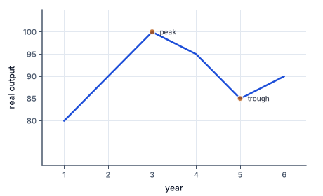
The figure plots this sequence, with the peak and the trough read from neighboring years.
Consider annual actual output values of eighty, ninety, one hundred, ninety-five, eighty-five, and ninety base-year dollars. In this supplied sequence, activity expands through the third observation, contracts through the fifth, and expands again at the sixth. The third observation is a local peak and the fifth a local trough. These labels compare neighboring observations under the problem's simplified rule; they do not claim that one short series implements an official recession-dating procedure.
Business cycles are not regular waves with a fixed period or amplitude. The word cycle describes recurring types of movement, not a mechanical schedule guaranteeing that a peak follows a set number of months after a trough. A diagram drawn as a smooth wave is a teaching illustration. It should not be mistaken for a fitted forecasting law or a promise that the next turning point can be read from elapsed time alone.
A downturn in one industry need not imply an economy-wide contraction. A broad assessment of aggregate activity may use output, employment, income, sales, and other measures, with attention to coverage and timing. Nor does a statistical agency's annual growth figure necessarily describe every quarter within the year. An annual average can rise even if activity fell near the end, depending on the path through the period.
The familiar rule of two consecutive quarters of declining real GDP is a shortcut, not a universal definition of recession across institutions and countries. The classification can depend on a broader set of indicators and a dating methodology. Our exercises avoid grading a contested real-time label from insufficient information: they state the turning-point rule or provide the cycle classification and ask what follows from it.
Seasonal patterns require separate attention. A tourism region can have lower measured activity every winter without each seasonal decline representing a new aggregate recession. A comparison should identify whether data have been seasonally adjusted and whether the question concerns seasonal variation or a broader cycle. In the fictional tables, seasonal effects are absent unless specified, so the learner can focus on the direction and level comparisons.
Potential output depends on productive capital, labor input under sustainable conditions, productivity, and the economic structure. It can grow as technology improves or the effective workforce expands. It can also be revised downward after durable damage to productive capacity. Holding potential fixed is a useful introductory comparison, but it is an assumption rather than a universal property of business-cycle analysis.
Suppose actual output is 960 base-year dollars. Under a potential estimate of one thousand, the gap is negative four percent. If new evidence revises potential to 960, the estimated gap becomes zero without any new production occurring between the two calculations. The output record has not changed; the benchmark has. A report attributing the entire revision to a sudden recovery would confuse a change in estimated capacity with a change in observed activity.
Potential is not directly observed in the way a completed transaction is recorded. Statistical and structural methods infer it using data and assumptions, and different methods can give different results. That uncertainty matters for policy analysis because a response suited to a demand-driven gap may differ from one addressing a persistent supply loss. The classroom's supplied potential figure makes a calculation gradeable; it does not remove the real-world estimation question.
The output gap often correlates with cyclical unemployment in aggregate models: below-potential production tends to accompany underused labor, other things equal. The relationship is not a universal fixed conversion between output percentage points and unemployment percentage points. Productivity, hours, participation, and labor retention can change how firms adjust. If an exercise supplies a particular coefficient, that coefficient belongs to its stipulated model, not to all economies at all times.
An economy can return to zero gap because actual output rises, potential falls, or both. These routes have different implications for productive capacity and living standards. The gap measures proximity to a benchmark, not the desirability of the benchmark itself. A smaller gap following destruction of capital does not establish an improvement in welfare. Always report the actual and potential levels alongside the percentage when the mechanism matters.
A leading indicator is one that has tended to move ahead of a chosen reference measure in a particular empirical setting. New orders may precede production, for example, because firms schedule work after receiving orders. That mechanism makes the indicator potentially informative, but orders can be canceled and the relationship can change. A leading indicator is not a logically sufficient condition for a future expansion or contraction.
A lagging indicator adjusts after the reference movement. Some employment measures may respond slowly because firms wait before hiring or dismissing workers, or because contracts and matching take time. A lag does not make the measure useless. It may confirm a change already suggested elsewhere or describe consequences that matter independently. Its timing must match the question being asked.
Coincident indicators move approximately with the reference cycle measure, but even this classification depends on the data frequency, period, and institution. Avoid assigning an immutable timing label to every variable. The assessed cases explicitly stipulate a timing relationship and ask the learner to interpret the evidence under that relationship. They do not ask for an actual forecast of a real economy.
Revisions complicate real-time interpretation. A preliminary output estimate may later change when fuller information arrives. An analyst at the earlier date could not have known the revised value, so evaluating a real-time decision requires preserving the information set available then. A smooth historical graph can conceal uncertainty that was substantial during the episode. Distinguish a retrospective description from an ex ante prediction.
Several agreeing indicators can strengthen an interpretation, but their independence matters. Three measures derived from the same underlying survey do not necessarily supply three independent confirmations. Likewise, a single summary index can combine components whose weights affect the signal. Ask which observations support the conclusion, what alternative explanations remain, and whether the inference is proportional to the evidence.
The course uses fictional time paths to practice these distinctions. A calculation of the supplied output gap is a model result. A claim that a real central bank should change rates, or that a recession will occur next quarter, would require additional evidence, uncertainty assessment, and decision criteria. The purpose of this lesson is to make those missing steps visible while teaching the exact comparisons that precede them.
A fictional statistical office reports actual real output of nine hundred base-year dollars in period one and 960 in period two. Its initial potential estimate is one thousand for both periods. The period-one gap is negative ten percent and the period-two gap is negative four percent. Actual production increased by sixty dollars, or approximately 6.67 percent relative to the earlier actual level. The economy recovered in this supplied sequence but initially remained below estimated potential.
The office then revises period-two potential downward to 960 after incorporating evidence of a lasting capacity loss. Under the revised estimate, the period-two gap is zero. Actual period-two output remains 960. The gap narrowed partly because output rose between periods and partly because the estimated sustainable benchmark changed. Those are different comparisons and should appear separately in an explanation.
A headline says the revision proves that all unused resources returned to work. That conclusion does not follow. The gap calculation does not identify each worker's status, hours, or reason for nonparticipation. Nor does zero gap mean zero unemployment in the introductory natural-rate model. A complete labor-market account needs the classifications and flows taught in the preceding lesson.
The corrected report can display actual output, old potential, revised potential, and both gap estimates. It can describe the actual output increase without claiming that the capacity loss was beneficial. This format preserves the evidence needed to compare two explanations: stronger current production versus a lower benchmark. It also makes clear why a smaller estimated gap is not automatically an improvement in living standards.
Positive actual growth does not imply a positive output gap. A falling estimated gap can reflect revised potential rather than new production. A peak is not necessarily above potential, and a trough is not defined by the lowest conceivable output. Business cycles have no fixed schedule. A leading indicator supplies evidence rather than a guaranteed forecast.
Record the two actual output levels.
Actual output rises from nine hundred to 950 base-year dollars.
This comparison identifies the direction of current activity.
Record same-date potential for the later period.
Potential output is one thousand base-year dollars.
The gap requires a capacity benchmark for the same period.
Subtract potential from actual output.
950 - 1,000 = -50 base-year dollars.
A negative difference places actual output below the supplied benchmark.
Scale the difference by potential.
-50/1,000 × 100 = -5%.
Potential, rather than earlier actual output, is the gap denominator.
State both comparisons without conflating them.
Actual output rose, while the later gap remains negative five percent.
Recovery and below-potential production can coexist.
Read the observations in time order.
80, 90, 100, 95, 85, 90 base-year dollars.
A turning point is defined relative to surrounding observations.
Identify the initial increases.
Output rises through observation three.
The first two interval changes are positive.
Identify the subsequent decreases.
Output falls from observation three through observation five.
The sign of the change reverses after the third observation.
Mark the renewed increase.
Observation six is above observation five.
The sign reverses again after the fifth observation.
Report the local turning points.
Peak at observation three; trough at observation five.
These labels follow the supplied sequence, not a claim of an official recession date.
Record the initial-period comparison.
Actual 900, potential 1,000: gap -10%.
Both levels refer to period one under the initial benchmark.
Record period-two actual output.
Actual 960 base-year dollars.
The observed output increase is sixty dollars regardless of a potential revision.
Calculate period two with the old benchmark.
(960 - 1,000)/1,000 = -4%.
Holding the benchmark fixed isolates the effect of the actual recovery.
Apply the revised capacity estimate.
Revised period-two potential 960.
The revision concerns the benchmark rather than an additional output observation.
Recalculate the revised gap.
(960 - 960)/960 = 0%.
The zero gap follows from equality of actual and revised potential.
Limit the interpretation.
Zero revised gap does not establish restored capacity or zero unemployment.
A lower benchmark can close a gap without reversing the underlying capacity loss.
Record the stipulated output values.
Actual 108, potential 100 base-year dollars.
The benchmark describes sustainable conditions in this model.
Calculate the gap.
(108 - 100)/100 = 8%.
Actual output is above the supplied potential level.
Interpret a subsequent actual decline to 104.
A fictional economy has actual real output 920 and potential real output 1,000 base-year dollars in period one, followed by actual 960 and potential 1,000 in period two. Compute the level gap and percentage gap in each period.
| Gap base-year dollars | Gap percent of potential | |
|---|---|---|
| Period one | ||
| Period two |
A fictional economy's real output rises from 400 to 440 base-year dollars. Later-period potential is 500. Complete actual growth and the later output gap.
Compute actual growth relative to the earlier observation.
Actual growth = growth percent.
The earlier actual output is the growth denominator.
Compare the later actual level with potential.
Actual minus potential = difference base-year dollars.
Both values refer to the later period.
Scale the gap by potential.
Later output gap = gap percent.
The potential benchmark supplies the denominator for this different comparison.
Plot a fictional real-output sequence with time on the horizontal axis: period one output eighty, period two ninety, period three seventy, period four eighty base-year dollars. Plot exactly those four observations.
Plot your answer on the grid:
A fictional economy's actual real output is 720 base-year dollars. An initial report estimates potential at 800; a revised report estimates it at 750. Actual output is unchanged. Compute each percentage output gap.
| Gap percent | |
|---|---|
| Initial estimate | |
| Revised estimate |
Construct the bounded argument about a fictional leading indicator. The case says new orders often precede production, but orders can be canceled.
This task has no paper form; do it on a device.
A fictional island produces 450 base-year dollars before and after a storm. Estimated sustainable capacity falls from 500 to 450 because equipment is permanently damaged. Compute the output gap percentage before and after, plus the change in actual output.
| Value | |
|---|---|
| Earlier gap percent | |
| Later gap percent | |
| Actual output change dollars |
Lesson test: one question per skill, one attempt each, no hints. Your answers are checked when you submit.
A fictional economy's actual real output is 800 then 880 base-year dollars. Potential is 1,000 in both periods. A later revision changes only second-period potential to 880. Compute actual growth percent, the second-period gap under the original potential estimate, and its gap under the revision.
| Percent | |
|---|---|
| Actual output growth | |
| Original second-period gap | |
| Revised second-period gap |
You can separate actual output changes from benchmark revisions and describe a recovery that still leaves output below potential. Next, model the spending relationships that form aggregate demand.
13. Growth with a positive gap, step 3
Output falls, but the gap remains positive four percent if potential stays 100.
A contraction in actual activity does not require the level to have already fallen below potential.