Back to the on-screen lesson ·
Construct conditional Phillips curves and distinguish monetary identities from causal predictions.
Paper packet. Every task here also exists on screen, where it is checked automatically; answers written on paper are not assessed by Nydus. When you are back at a device, enter your answers there.
Calculate and plot Phillips-curve points, separate movements from expectations and supply shifts, derive a conditional long-run unemployment result, and apply exact quantity-equation growth with explicit assumptions.
Aggregate demand can change output when nominal adjustment is incomplete, while expected inflation affects real financing costs. These ideas also matter for the relationship between inflation and unemployment. A Phillips-curve exercise is a conditional model with expectations, supply conditions, and a natural unemployment rate. It is not an instruction to choose any permanent inflation-unemployment pair.
| Term | What it means |
|---|---|
| Expected inflation | The inflation rate anticipated for the relevant future interval. |
| Short-run Phillips curve | A conditional relationship between inflation and unemployment for given expectations and supply conditions. |
| Natural unemployment rate | A model's unemployment rate consistent with its structural and frictional conditions in long-run equilibrium. |
| Velocity | Nominal expenditure on final output divided by the defined money stock over the stated period. |
| Monetary neutrality | A model property under which a nominal monetary change leaves long-run real quantities unchanged under its assumptions. |
A simple short-run Phillips curve can be written π = πe - b(u - un) + s. Inflation π depends on expected inflation πe, the difference between unemployment u and its natural rate un, a positive responsiveness coefficient b, and a supply-shock term s. When the exercise measures rates in percentage points, a value of four means four percent, not the decimal 0.04. State this convention before substituting.
Holding expected inflation, the natural rate, and the supply term fixed, lower unemployment corresponds to higher inflation in this model. That is a movement along one short-run curve. An increase in expected inflation shifts the whole relationship upward. An adverse supply shock represented by a higher s also raises inflation at a given unemployment rate, but it has a different source and can require a different adjustment account.
The distinction prevents a common inference error. Observing unemployment and inflation rise together does not refute every conditional Phillips-curve model: a shift can dominate the movement along a curve. Nor does a fitted inverse association prove that policy can exploit a stable permanent trade-off. The model's expectations and structural parameters must remain relevant to the question being answered.
Another way: steps
Label actual inflation, expected inflation, unemployment, the natural rate, and the supply term. Calculate a point using the supplied equation. For a comparison, identify which parameter changes. Use long-run equality of actual and expected inflation only when explicitly assumed, and keep nominal identities separate from causal theories.
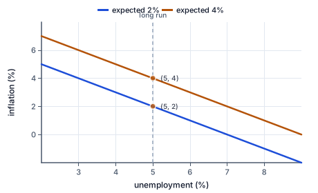
The figure draws both curves of this example: higher expected inflation lifts the whole curve, a shift rather than a movement along it.
Take a fictional curve π = 2 - (u - 5), with all rates in annual percentage points. Expected inflation is two percent, the natural unemployment rate is five percent, the slope coefficient is one, and the supply term is zero. At unemployment of five percent, inflation equals two percent. At unemployment of four percent, inflation equals three percent. At unemployment of six percent, inflation equals one percent.
These points form one downward-sloping relationship when unemployment is horizontal and inflation is vertical. A change from unemployment of five to four along this curve raises inflation by one percentage point. The equation alone does not identify the policy or demand disturbance that produced the movement. A separate aggregate-demand mechanism can supply that explanation, but the graph itself records a conditional relationship.
If expected inflation rises from two to four percent while the natural rate and supply term stay fixed, the new curve is π = 4 - (u - 5). At every unemployment rate it lies two percentage points above the original curve. At unemployment of five, inflation is now four. This is a shift, not movement along the old curve. Keeping the original intercept while verbally claiming expectations changed would produce an inconsistent model.
Alternatively, hold expectations at two and add a supply-shock term of two. The numerical curve is again π = 4 - (u - 5), but the interpretation differs. One case has revised expectations; the other has a supply disturbance. The same observed pair can therefore be consistent with multiple mechanisms. Distinguishing them requires information beyond the pair's coordinates, such as the problem's stated shock or evidence about wage setting and input costs.
The natural rate can also change if structural or frictional conditions change. It is neither necessarily constant nor directly observed without uncertainty. Different estimation methods and later data revisions can yield different estimates. In an exercise it is a supplied model parameter. In an empirical discussion, treating one estimate as an exact threshold can conceal uncertainty relevant to the policy judgment.
Suppose a long-run comparison assumes the supply-shock term has returned to zero and actual inflation equals expected inflation. Substituting these conditions into π = πe - b(u - un) leaves b(u - un) = zero. With positive b, unemployment equals the natural rate. Different sustained inflation rates can then correspond to the same long-run unemployment rate, producing a vertical long-run Phillips curve in this model.
The derivation does not claim that inflation has no costs or that every economy always sits at its natural rate. It identifies a model restriction under which systematically surprising wage and price setters is not a permanent source of lower unemployment. Adjustment can take time, contracts can be staggered, and disturbances can persist. The path to the long-run comparison needs its own assumptions about expectations and nominal adjustment.
If a demand expansion temporarily lowers unemployment below the natural rate while expectations are fixed, actual inflation exceeds expected inflation under the equation. If expectations later adjust upward, the short-run curve shifts. Maintaining the same low unemployment would then require still higher inflation in this simple adaptive account. That conditional sequence differs from a one-time permanent reduction in unemployment purchased at a fixed inflation rate.
An anticipated credible change in policy may alter expectations earlier than an adaptive rule would suggest. A disinflation can therefore have different transitional output and employment costs under different expectations, credibility, rigidity, and shock assumptions. A sacrifice ratio calculated from one episode is not automatically a universal constant. The course assesses the stated mechanisms and arithmetic, not a claim that one policy announcement guarantees costless adjustment.
Stabilization objectives can conflict after an adverse supply shock because the shock raises inflation pressure while reducing output. A demand contraction may reduce inflation pressure while worsening the short-run output gap. A demand expansion may support activity while adding inflation pressure. Model comparison should identify these conditional trade-offs and the horizon, rather than presenting a curve as a complete policy recommendation.
The long-run curve's verticality also does not imply that structural policies can never affect employment. Education, matching, mobility, institutions, and other conditions may change the natural-rate parameter or productive capacity through separate mechanisms. Whether a particular intervention does so requires evidence and a model of those mechanisms. Moving the parameter differs from trying to remain forever below an unchanged parameter through unanticipated nominal demand.
The equation MV = PY relates a defined money stock M, its velocity V, a price level P, and real output Y. When velocity is defined as nominal final expenditure PY divided by M, the equation holds by construction. It does not alone show that changing money causes an equal proportional change in prices. To make that causal prediction, one needs additional assumptions about velocity, real output, the policy mechanism, and the adjustment horizon.
In a fictional long-run quantity-theory comparison, suppose velocity is fixed and real output is fixed at its potential level. If the money stock rises by ten percent, nominal expenditure rises by ten percent and the price level rises by ten percent. This is a valid implication of those supplied assumptions. If real output instead rises by ten percent as well, the same money increase with unchanged velocity can leave the price level unchanged.
For exact growth arithmetic, use gross growth factors. The price-level factor equals the money-stock factor multiplied by the velocity factor and divided by the real-output factor. If money grows by twenty percent, velocity is unchanged, and real output grows by ten percent, the price factor is 1.20 divided by 1.10. Inflation is approximately 9.09 percent, rather than exactly ten percent. The common growth-rate subtraction is an approximation, not an identity at large rates.
A simpler exact example uses money growth of twenty-five percent and output growth of twenty-five percent with fixed velocity. Both factors are 1.25, so the price factor is one and inflation is zero. Another exact comparison uses money growth of fifty percent and output growth of twenty percent: 1.50 divided by 1.20 is 1.25, giving inflation of twenty-five percent. These examples make the multiplicative relationship visible.
Velocity can change with payment technology, desired liquidity, financial conditions, and the definition of the money aggregate. Broad money itself can respond endogenously to credit and spending conditions. Consequently, a correlation between a monetary aggregate and nominal expenditure does not by itself identify an exogenous policy experiment. The declared quantity-theory exercise holds particular components fixed to isolate one mechanism.
Monetary neutrality is similarly a model property with a horizon and assumptions, not a claim that monetary disturbances never affect real activity. A model can allow short-run real effects through sticky wages and prices while predicting a different long-run comparison after adjustment. Persistent financial disruption, changing expectations, and effects on investment may require richer analysis. State what the simple model concludes, what assumptions generate that conclusion, and what remains outside its scope.
A fictional economy initially follows π = 2 - (u - 5), with rates in annual percentage points. An analyst later observes unemployment of five percent and inflation of four percent. The old curve predicts only two-percent inflation at that unemployment rate, so the observed point requires a changed condition if this model is retained.
One proposed explanation raises expected inflation from two to four percent with no supply shock. Another keeps expected inflation at two percent but adds a supply term of two percentage points. Each produces π = 4 - (u - 5), and each predicts four-percent inflation at unemployment of five. The numerical observation alone does not distinguish the two stories.
The analyst should request evidence about the changed condition rather than infer it solely from the graph. Measures of expectations, wage contracts, input disruptions, and other relevant information may help assess the explanations, but each measure has limits. A model exercise can simply state which mechanism occurred; an empirical explanation must justify the choice with evidence.
For a long-run comparison, suppose the supply disturbance disappears and expectations settle at actual inflation. With the natural rate still five, the simple model puts unemployment at five percent regardless of whether the stable inflation rate is two or four percent. This does not make those inflation outcomes equally desirable or guarantee a painless transition. It establishes the conditional vertical long-run relationship and shows why a short-run curve cannot be treated as a permanent menu independent of expectations.
A movement along one short-run curve holds expectations and supply conditions fixed. Changes in those conditions shift it. A vertical long-run curve follows additional equilibrium assumptions and does not deny transitional real effects. MV=PY is an identity with defined velocity; a proportional money-to-price prediction additionally fixes velocity and real output.
Write the complete supplied relationship.
π=2-(u-5), rates in percentage points.
The intercept embeds expected inflation and the natural rate is specified separately.
Insert the observed unemployment rate.
u=4%.
Unemployment is the horizontal coordinate in this graph.
Compute the unemployment gap.
u-un=4-5=-1 percentage point.
The economy is below the supplied natural rate.
Calculate the predicted inflation rate.
π=2-(-1)=3%.
Subtracting a negative gap raises inflation above expectations in this model.
Identify the maintained conditions.
Expected inflation2%, natural rate5%, supply termzero.
The calculated point belongs to this conditional curve only while those parameters remain fixed.
Record the original expectations parameter.
πe=2%, un=5%, b=1, s=0.
The starting curve distinguishes expectations from the unemployment gap.
Change only expected inflation.
New πe=4%.
The case holds the natural rate, slope, and supply conditions fixed.
Write the new relationship.
π=4-(u-5).
An expectations change shifts the conditional inflation schedule.
Evaluate both curves at unemployment five.
Old inflation2%; new inflation4%.
A common unemployment coordinate isolates the shift.
State the vertical displacement.
The curve shifts upward two percentage points.
Every point changes by the same amount because only the expectations intercept changed.
Record the nominal accounting relationship.
MV=PY.
With defined velocity, the equation alone is an identity.
State the comparison's behavioral assumptions.
Velocity is fixed; real output rises twenty percent.
These conditions supply information not contained in the identity alone.
Record the money-stock change.
Money grows fifty percent, so its factor is1.50.
Exact proportional calculations use gross factors.
Calculate the price-level growth factor.
Price factor=1.50×1÷1.20=1.25.
Real-output growth absorbs part of the nominal-expenditure growth.
Convert the factor into inflation.
Inflation=(1.25-1)×100=25%.
The result is a percent change in prices rather than the price factor itself.
Limit the causal interpretation.
The result depends on fixed velocity and the supplied real-output path.
Changing either assumption changes the implication even while the identity continues to hold.
Set actual and expected inflation equal.
π=πe and the supply term iszero.
These are explicit long-run conditions rather than facts about every observed quarter.
Cancel the equal inflation terms.
0=-b(u-un).
Only the unemployment-gap component remains in the supplied relationship.
Use the positive slope coefficient.
A fictional short-run curve is π=3-(u-5), with inflation and unemployment measured in annual percentage points. Compute inflation at unemployment four and six percent, holding all curve parameters fixed.
| Inflation percent | |
|---|---|
| u=4 | |
| u=6 |
In a fictional exact quantity-equation comparison, money grows fifty percent, velocity is unchanged, and real output grows twenty percent. Complete the gross money factor, gross output factor, and resulting inflation rate.
Convert the money change into a gross factor.
Money factor=money.
A growth factor includes the initial stock as well as its proportional increase.
Convert the real-output change into a gross factor.
Output factor=output.
The output factor belongs in the denominator when solving for price growth.
Divide the factors and convert back to a rate.
Inflation=inflation percent.
Exact multiplication and division replace the approximate subtraction of growth rates.
Plot the fictional short-run Phillips curve π=4-(u-5) at unemployment u=3,5,7 percent. Unemployment percent is horizontal; annual inflation percent is vertical.
Plot your answer on the grid:
Two fictional Phillips curves have natural unemployment5%, slope coefficientone, and zero supply shock. Expected inflation is2% in A and5% in B. Compute inflation in each at unemployment4%, then the vertical difference B minus A. Rates are annual percentage points.
| Value | |
|---|---|
| A inflation percent | |
| B inflation percent | |
| Vertical difference percentage points |
Construct the stated model argument. The Phillips equation is π=πe-b(u-un)+s with b>0. The long-run comparison assumes actual equals expected inflation and the supply term is zero. Link the joint conditions to cancellation, then the resulting unemployment equality and vertical long-run curve.
This task has no paper form; do it on a device.
A fictional payments report shows money stock200 dollars, real output100 units, and price leveltwo dollars per unit. In a later period money is250, output remains100, and velocity stays at its initial value. Compute initial velocity, later nominal expenditure, and later price level.
| Value | |
|---|---|
| Initial velocity per period | |
| Later nominal expenditure dollars | |
| Later dollars per output unit |
Lesson test: one question per skill, one attempt each, no hints. Your answers are checked when you submit.
A fictional Phillips model is π=πe-2(u-un)+s, with all rates in annual percentage points and un=5. Initially πe=2 and s=0. Compute inflation at u=4. Next hold u=4 but raise πe to4 and s to1. Compute the new inflation and its change. Finally, for a separate long-run comparison assume s=0 and π=πe; give the implied unemployment rate.
| Value | |
|---|---|
| Initial inflation percent | |
| New inflation percent | |
| Inflation change percentage points | |
| Long-run unemployment percent |
You can explain why expectations and supply conditions change inflation-unemployment comparisons and why a monetary identity alone is not a causal theory. Next, examine the productive capacity that determines long-run growth.
13. Derive the model's long-run unemployment, step 3
With b>0, u=un.
The model permits different stable inflation rates at the same natural unemployment rate.