Back to the on-screen lesson ·
Distinguish stock and flow markets and compare conditional financing responses.
Paper packet. Every task here also exists on screen, where it is checked automatically; answers written on paper are not assessed by Nydus. When you are back at a device, enter your answers there.
Construct fixed-supply money-market and real loanable-funds equilibria, plot declared saving points, and reconcile partial crowding out without confusing nominal rates, real rates, or deficit-accounting conventions.
Bank balance sheets distinguish deposits from reserves, while bond pricing relates dated payments to yields. Two common macroeconomic diagrams now organize different financial questions. The money market concerns desired money balances, and the loanable-funds model concerns saving and borrowing flows. Label quantities, time, and the nominal or real interest rate before comparing them.
| Term | What it means |
|---|---|
| Money demand | Desired holdings of the defined money balance under stated transaction and portfolio conditions. |
| Opportunity cost of holding money | The return forgone relative to a specified interest-bearing alternative. |
| Loanable funds | A model of saving supplied and borrowing demanded over a period. |
| Real interest rate | An interest rate adjusted for expected or realized inflation according to the model's timing. |
| Crowding out | A reduction in some private spending induced by a policy or financing change through a specified mechanism. |
A simple money-market diagram puts the nominal interest rate vertically and a stock of money balances horizontally. Money demand represents how much of the defined liquid asset people want to hold, not how much income they want to earn. If money pays less interest than an alternative asset, a higher alternative yield raises the opportunity cost of holding it, other things equal. This can give money demand a negative relationship with the nominal rate.
A loanable-funds diagram instead places a real interest rate vertically and a flow of funds per period horizontally. Saving supplies funds in the specified model, while investment or other borrowing demands them. A higher real rate can encourage saving and discourage some investment projects, creating an upward supply relationship and downward demand relationship. These slopes are supplied behavioral assumptions, not accounting identities.
Calling both diagrams a market for money conceals the distinction. A stock of transaction balances at a date is not the same as dollars of saving per year. A nominal opportunity cost is not automatically the same as a real borrowing cost. The diagrams can be linked in a broader model, but one cannot be substituted for the other merely because both show a rate on the vertical axis.
Another way: steps
Name the horizontal quantity, its stock or flow units, and the interest-rate definition. Write the supplied demand and supply relationships. Solve their equality. For a policy comparison, change only the relationship the model says is affected and trace any offset separately.
Suppose real money demand is L = 200 - 20i, where L is real money balances in base-year dollars and i is a nominal annual rate measured in percentage points. A rate of five means five percent in this equation, not the decimal 0.05. If the model supplies real money balances of one hundred, equilibrium requires 100 = 200 - 20i, so i = five percent.
If the nominal money stock rises while the price level stays fixed, real supplied balances rise. With real supply of 120 and unchanged demand, the rate is four percent. This is a movement along the given demand relationship caused by a change in the supplied quantity. It is a valid comparison in a model with an exogenously specified money stock and the stated adjustment mechanism. It is not automatically the description of an ample-reserves central bank targeting an administered rate.
Money demand can shift when real income or transaction needs change. If people conduct more transactions at a given rate, desired balances can rise. A change in payment technology or preferences for liquidity can also alter the relationship. The shift's size and direction should be stated or justified, rather than assumed from a vague claim that people want more money. Wanting more purchasing power is not the same as choosing to hold a larger share of wealth in a particular liquid asset.
The rate relevant to money holding can be a spread between the return on money-like assets and a competing return. If deposits themselves pay interest, their opportunity cost is not simply the full yield on another instrument. Risk, transaction services, and access restrictions can also matter. The elementary downward curve simplifies these features. A careful explanation identifies which asset counts as money and which return is being forgone.
When a central bank targets a short-term rate, the quantity adjustment may be different from the vertical fixed-supply diagram. The bank can accommodate demand for settlement balances or use administered rates under an ample-reserves framework. The following lesson compares those implementations explicitly. The current exercise teaches how to solve one declared money-market model without claiming that its instrument choice is universal.
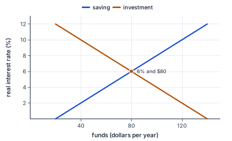
The figure draws these schedules, crossing at six percent and eighty dollars a year.
Consider fictional annual saving S = 20 + 10r and private investment demand I = 140 - 10r, where r is a real annual interest rate in percentage points and flows are dollars per year. Equating gives 20 + 10r = 140 - 10r, so r = six percent and the funds flow is eighty dollars per year. Substitution into both relationships verifies the same quantity.
The upward saving schedule represents a stipulated net response. In a richer household model, a higher return has substitution and income effects that can work differently for savers and borrowers. The downward investment schedule reflects fewer projects meeting a higher financing or opportunity-cost threshold, holding expected returns and other conditions fixed. Neither slope should be presented as a theorem applying unchanged in every episode.
An improvement in expected project profitability can shift investment demand right. A change in household saving preferences can shift saving supply. International capital flows can add another margin of adjustment in an open economy. Comparing these events requires preserving the model's definition of the funds market and whether the supply includes foreign financing. A closed-economy result need not carry over unchanged when cross-border flows are allowed.
The real rate definition also needs its inflation assumption. If expected inflation is fixed, a change in the relevant nominal borrowing rate changes the expected real rate correspondingly under the specified approximation or exact formula. If expected inflation changes too, the real-rate response cannot be read from the nominal movement alone. Earlier lessons supplied the exact purchasing-power relationship; use a consistent convention here.
This saving-investment model abstracts from the detailed bank balance sheets that create and settle deposits. It organizes a macroeconomic allocation relationship, not a claim that each commercial loan can only occur after one named household deposits an equal amount of prior saving. The balance-sheet account and the loanable-funds comparison answer different questions. Connecting them requires an explicit broader model rather than using one to erase the other.
In one convention, the supply curve represents private saving, and total demand for funds includes private investment plus government borrowing. Starting from S = 20 + 10r and I = 140 - 10r, add government borrowing of forty dollars per year. Total demand is 180 - 10r. Equilibrium becomes r = eight percent, with total funds of one hundred. Private investment at that rate is sixty, so it falls by twenty relative to the original eighty.
The forty-dollar government borrowing is partly matched by twenty dollars of additional private saving and partly by twenty dollars of reduced private investment in this model. It does not crowd out forty dollars of investment because the saving supply is responsive. A vertical saving schedule would produce a different division; monetary accommodation, idle resources, or foreign financing could change the response further. The magnitude follows from the stated relationships.
Another common convention uses national saving as supply and private investment as demand. A government deficit can reduce national saving at a given rate, shifting the supply curve left. This can represent the same financing pressure with different curve labels. Do not shift national saving left and also add the same government borrowing to demand unless the model explicitly defines distinct changes. Otherwise the same deficit is counted twice.
Crowding out is not limited to one financial diagram, but every use of the term needs a mechanism. Higher interest rates can reduce interest-sensitive spending in the model above. Exchange-rate appreciation can affect net exports in an open-economy mechanism. Resource constraints can redirect labor and materials. These channels should be distinguished, and none establishes that a policy is desirable or undesirable without its other effects and objectives.
The model is a comparative-static account of equilibrium flows. It does not specify how fast rates or saving adjust, whether credit is rationed, or how banks reprice different loans. It also does not prove that a deficit observed during a recession caused the recession's investment decline. Both can respond to weaker activity. Causal interpretation needs a defined counterfactual and evidence about the proposed channel.
Useful disagreement analysis asks what is held fixed. Two analysts can obtain different investment responses because one assumes fixed saving and another allows saving to rise, because one permits capital inflows, or because they use different monetary responses. Identifying those assumptions permits a fair model comparison. It is more precise than treating one diagram as a universal answer to every fiscal-financing question.
A fictional annual funds market has private saving S = 20 + 10r and private investment I = 140 - 10r, where r is the real annual rate in percentage points. Initially the government does not borrow in this model. Equilibrium is r = six percent and both saving and investment are eighty dollars per year. The case then adds forty dollars of government borrowing, holding the private schedules and all other conditions fixed.
Under the private-saving convention, total borrowing demand becomes I + 40 = 180 - 10r. Setting this equal to saving gives r = eight percent and total funds of one hundred dollars. Private investment is now 140 - 80 = sixty dollars, while government borrowing is forty. The two uses add to the one-hundred-dollar saving flow, so the ledger reconciles.
A headline claims that every dollar borrowed by government displaced a dollar of private investment. The supplied schedules do not support that claim: private investment fell twenty dollars, not forty. Private saving increased by twenty as the rate rose. A different model with a fixed saving quantity could produce complete displacement, but that is not the stated model.
The correction should identify the real-rate change, the total funds flow, the private-investment response, and the saving response separately. It should also note that this is a closed-model comparison with unchanged private relationships. Allowing foreign capital flows, a different monetary response, or changes in expected project profitability would require a new set of equations. The calculation is a conditional mechanism, not a verdict on government borrowing.
Money demand is desired asset holding, not demand for income. Money balances are a stock; saving and borrowing are flows. Nominal and real rates require consistent inflation assumptions. A bank's ability to create deposits does not remove funding and risk constraints. Do not represent one deficit as both a national-saving reduction and an added borrowing demand unless the model defines separate effects.
State the demand rule and rate units.
L=200-20i; i is nominal annual percentage points.
Using 0.05 instead of five would change the meaning of the supplied coefficients.
Record real supplied money balances.
Real supply is one hundred base-year dollars.
The problem fixes the quantity rather than the interest rate.
Equate desired and supplied balances.
100=200-20i.
Equilibrium requires the public to willingly hold the supplied stock.
Solve the rate.
20i=100; i=5%.
The solution follows the demand schedule's stated units.
Check the demand value.
200-20×5=100.
The desired stock matches the supplied stock at the calculated rate.
State saving and investment schedules.
S=20+10r; I=140-10r dollars per year.
Both quantities are flows over the same annual interval.
Equate the two planned flows.
20+10r=140-10r.
The supplied closed model requires saving to fund the investment flow.
Solve for the real rate.
20r=120; r=6%.
The rate is measured in percentage points in these equations.
Calculate the flow from saving.
S=20+60=80 dollars per year.
The equilibrium rate determines the supplied funds flow.
Verify the flow from investment.
I=140-60=80 dollars per year.
Agreement verifies that the same rate clears both sides.
Record the original equilibrium.
Real rate 6%; private saving and investment eighty dollars per year.
The initial schedules provide a common comparison point.
Add government borrowing to total demand.
Total demand=180-10r.
This convention uses private saving as supply, so the new borrowing belongs on demand.
Solve the shifted equilibrium.
20+10r=180-10r; r=8%.
The same private-saving schedule responds to the higher rate.
Calculate total saving and private investment.
Saving 100; private investment 60 dollars per year.
The government and private sector are separate users of the funds flow.
Reconcile the additional borrowing.
Forty government borrowing equals twenty extra saving plus twenty displaced private investment.
The response is partial crowding out because saving supply is not fixed.
State the convention and limits.
Do not also shift national saving for the same deficit in this representation.
Changing the model's accounting convention requires redefining its curves rather than duplicating the event.
Keep money demand unchanged.
L=200-20i.
The comparison holds income and the preference for liquidity fixed.
Raise real supplied balances to 120.
120=200-20i gives i=4%.
The changed quantity moves along the given demand relationship.
Name the scope of the rate result.
A fictional fixed-supply money market has real money demand L=180-20i, with i a nominal annual rate in percentage points. Compute equilibrium i for real supplied balances of one hundred and 120 base-year dollars.
| Nominal rate percent | |
|---|---|
| Supply 100 | |
| Supply 120 |
A fictional annual funds market has private saving S=30+5r and investment I=110-5r. Government then adds twenty dollars of borrowing, so total demand becomes130-5r. Rates are real percentage points. Complete the new equilibrium.
Equate private saving with total borrowing demand.
New real rate=rate percent.
The government's borrowing is included only in the demand expression in this convention.
Evaluate total saving at the new rate.
Total funds=funds dollars per year.
The saving schedule supplies both private and government uses.
Evaluate private investment separately.
Private investment=investment dollars per year.
Subtracting government borrowing from the total gives the same private flow.
A fictional annual loanable-funds supply is S=20+10r, where r is the real rate in percentage points and S is dollars per year. Plot quantity horizontally and rate vertically at r=2,4,6.
Plot your answer on the grid:
A fictional closed annual funds model has S=40+10r and private I=160-10r, where r is real annual percentage points. Compute equilibrium r and the annual funds flow.
| Value | |
|---|---|
| Real rate percent | |
| Funds dollars per year |
Construct the stipulated funds-market mechanism. Private saving rises with the real rate, private investment falls with it, and government adds borrowing demand while the schedules stay fixed.
This task has no paper form; do it on a device.
A fictional project-finance market initially has S=20+10r and I=140-10r dollars per year. A separately stipulated foreign funds inflow adds forty to supply at every real rate, with no other changes. Compute the new real rate, total supplied funds, and private investment.
| Value | |
|---|---|
| New real rate percent | |
| Total funds dollars per year | |
| Private investment dollars per year |
Lesson test: one question per skill, one attempt each, no hints. Your answers are checked when you submit.
A fictional closed annual model has private saving S=30+10r and private investment I=150-10r, with r a real rate in percentage points. Government borrowing rises from zero to twenty dollars per year; private schedules do not change. Compute the new rate, total funds, private investment, and the change in private investment from the original equilibrium.
| Value | |
|---|---|
| New real rate percent | |
| Total funds dollars per year | |
| Private investment dollars per year | |
| Private investment change dollars per year |
You can identify the quantity and rate in each financial diagram and explain how assumptions determine the financing response. Next, compare central-bank implementation with limited and ample reserve balances.
13. More money balances under a fixed-stock regime, step 3
The nominal rate falls from five to four percent in this fixed-supply model.
An administered-rate operating regime needs a different implementation description.