Back to the on-screen lesson ·
Derive fixed-price spending responses and compare the assumptions behind fiscal mechanisms.
Paper packet. Every task here also exists on screen, where it is checked automatically; answers written on paper are not assessed by Nydus. When you are back at a device, enter your answers there.
Construct expenditure equilibria and fiscal multiplier comparisons, distinguish lump-sum taxes from proportional leakages, and identify automatic stabilizers and the conditions limiting real-world transfer of a model result.
A demand shift does not automatically translate dollar for dollar into equilibrium output because prices and other spending can respond. This lesson deliberately specifies a simpler fixed-price expenditure model to derive a multiplier. Its assumptions explain both the arithmetic and why the result should not be presented as an automatic real-world effect.
| Term | What it means |
|---|---|
| Marginal propensity to consume | The change in consumption associated with one additional unit of disposable income within the stated model. |
| Autonomous expenditure | Spending fixed independently of current income in the model. |
| Expenditure multiplier | The ratio of equilibrium output change to a specified autonomous spending change under the model's assumptions. |
| Lump-sum tax | A tax amount that does not vary with income within the exercise. |
| Automatic stabilizer | An existing fiscal rule that changes taxes or transfers as economic conditions change without a new discretionary decision. |
Assume a fictional closed economy has idle productive capacity, fixed prices, no income taxes or imports, and no interest-rate or expectation offsets. Households consume a constant share c of each additional dollar of income, while the remaining share is saved. Firms meet the additional demand by producing more. Under these assumptions, an extra government purchase of forty dollars becomes forty dollars of income, some of which supports another round of spending.
If c is 0.75, the next consumption round is thirty dollars, followed by 22.5 dollars, then 16.875 dollars, and progressively smaller rounds. The total approaches forty divided by one minus 0.75, or 160 dollars. The multiplier is four. The first forty dollars is included in that total; adding it again would double count the initial injection.
The rounds also need a common price basis and accounting period. Adding spending measured at changing prices would mix nominal valuation with real production, while counting the same transaction in two rounds would inflate the total. Each new round must be expenditure induced by income from an earlier round under the stated behavioral rule.
The ratio is not a claim that government creates physical resources from nothing. The model assumes unused productive capacity and a spending shortfall that firms can meet at fixed prices. If production cannot expand, if prices rise, or if other spending is displaced, the simple output result changes. The mechanism depends on repeated income-induced expenditure with limited leakage, not on the identity Y = C + I + G alone.
Another way: steps
State the consumption rule and all leakages. Write planned expenditure as a function of income. Solve Y equal to planned expenditure. Change only the specified autonomous term, solve again, and compare the equilibrium difference with the derived multiplier.
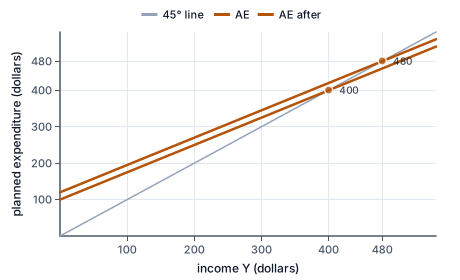
The figure draws this example: the expenditure line meets the 45-degree line at 400, and the twenty-dollar rise moves the crossing to 480.
Let planned expenditure be AE = A + cY, where A collects autonomous consumption, investment, and government purchases in this simplified closed economy. Equilibrium requires Y = A + cY. Moving the induced-consumption term gives (1 - c)Y = A, so Y = A/(1 - c). If A increases by a specified amount while c and all other conditions remain fixed, equilibrium output increases by that amount divided by one minus c.
With A equal to one hundred dollars and c equal to 0.75, equilibrium output is four hundred dollars. If A rises to 120, equilibrium becomes 480. The eighty-dollar increase is four times the twenty-dollar autonomous change. This algebra gives the same result as the infinite sequence of diminishing expenditure rounds, while avoiding a long list of individual rounds.
The marginal propensity is a response to an additional dollar, not the fraction of all income currently consumed. A household can consume a high average share of income while having a different marginal response to a temporary income change. Nor must every household have the same response in reality. The constant c is a deliberate simplification that makes the exercise determinate.
The condition that c is less than one matters for the convergent multiplier. At c equal to one with no other leakage, this simple setup has no finite stable adjustment to a positive autonomous injection using the displayed formula. That does not imply a real economy has infinite output. It means the specified assumptions no longer provide a finite equilibrium through this mechanism. Model breakdown should be identified rather than interpreted literally.
The model also distinguishes planned from unplanned investment. If planned expenditure initially falls below production, inventories can accumulate unexpectedly. Firms may reduce production in response, lowering income and consumption until the model reaches equilibrium. The realized expenditure identity remains satisfied through inventories throughout this story. It is the equality of planned expenditure and output that defines the fixed-price equilibrium here.
Introduce a lump-sum tax T and consumption C = a + c(Y - T). With investment and government purchases autonomous, the equilibrium equation becomes Y = a + cY - cT + I + G. A one-dollar tax increase directly reduces consumption by c dollars rather than by one dollar, because the model assumes households spread the disposable-income change between consumption and saving. The lump-sum tax multiplier is therefore -c/(1 - c).
If c is 0.75, the spending multiplier is four and the tax multiplier is negative three. Raising government purchases by twenty dollars increases model output by eighty. Raising lump-sum taxes by twenty lowers it by sixty. Doing both together raises output by twenty under this particular fixed-price, closed-economy setup. The resulting balanced-budget multiplier of one depends on the assumptions; it is not a universal description of every tax-financed spending program.
An income-dependent tax is different from a lump-sum amount. If disposable income is (1 - t)Y and consumption responds with marginal propensity c, induced domestic consumption contributes c(1 - t)Y. If imports also rise with income at rate m, the planned domestic-expenditure slope becomes c(1 - t) - m in a specified linear model. The corresponding multiplier is one divided by 1 - c(1 - t) + m, provided the model's stability conditions hold.
For example, c = 0.8, t = 0.25, and m = 0.1 give an induced domestic-spending slope of 0.5 and a multiplier of two. The simple no-tax, no-import multiplier at c = 0.8 would be five. The lower result does not mean the arithmetic is inconsistent. It reflects additional leakages from each income round under the more detailed assumptions.
An import leakage reduces the domestic output response in this model because some additional spending buys foreign production. It does not mean imported goods have no value or that preventing imports necessarily improves welfare. Similarly, saving is a leakage from the current consumption round, not a moral failure or a claim that saving never finances investment. The terminology describes this short-run expenditure model and must not be stretched into an unrestricted policy judgment.
Government purchases, taxes, and transfers can affect planned expenditure through different immediate channels. A purchase enters demand directly. A transfer changes disposable income, with consumption depending on the recipient's response. A tax change can alter disposable income and, in richer models, incentives and expectations. Treating all three as mechanically identical injections ignores those distinct links.
Automatic stabilizers operate through existing rules. During a downturn, tax receipts can fall as incomes fall, while some transfers rise as more people qualify. Relative to a fixed-tax, fixed-transfer comparison, these changes can cushion disposable income and spending without a new policy vote. In an expansion the same rules can work in the opposite direction. The strength of the effect depends on eligibility, responsiveness, and the spending response of recipients.
Discretionary policy involves a new decision, such as changing a purchase program or tax rule. Recognition, legislative, implementation, and spending-response lags can separate the initial shock from its eventual demand effect. A policy designed using an old output-gap estimate may arrive after conditions change. This is a reason to analyze timing and uncertainty, not a proof that all discretionary action succeeds or fails.
Interest rates and private investment can respond to fiscal changes. If government borrowing competes for a limited supply of saving in a stated loanable-funds model, higher rates can reduce private investment, offsetting part of the initial demand expansion. In a depressed economy with different monetary accommodation or saving responses, the offset can differ. The financial-sector lessons will identify these assumptions rather than treating crowding out as either always complete or never present.
Supply conditions also matter. With substantial idle capacity and sticky prices, the output response can be larger than near a binding productive constraint, where additional demand puts more pressure on prices. Expectations about future taxes or persistent policy changes can alter current behavior. A multiplier estimated in one episode need not transfer unchanged to another with different conditions.
The appropriate conclusion is conditional: under the supplied fixed-price model, a stated autonomous change produces the computed output change. Whether that model approximates an actual policy episode is an empirical question. Whether the policy is desirable also requires objectives, costs, distributional consequences, and alternatives. The course grades the derivation, the scope, and the identification of changed assumptions rather than agreement with a policy preference.
A fictional economy has consumption response c = 0.75, fixed prices, unused capacity, no imports, lump-sum taxes, and no interest-rate offsets. A proposal raises government purchases by twenty dollars and raises lump-sum taxes by twenty dollars in the same period. A report says the tax increase cancels the spending increase exactly, leaving aggregate demand and output unchanged.
In the stated model, the direct purchase adds twenty dollars of spending, while the tax change initially reduces consumption by fifteen dollars. The net autonomous injection is five dollars. Multiplying by four gives a twenty-dollar increase in equilibrium output. The same result follows by combining the eighty-dollar government-purchase effect with the negative sixty-dollar tax effect. Two routes provide a useful arithmetic check.
Now compare another model with c = 0.8, proportional income tax t = 0.25, and import propensity m = 0.1. Its induced domestic-spending slope is 0.8 times 0.75 minus 0.1, or 0.5. A separate twenty-dollar autonomous domestic-spending increase produces a forty-dollar output increase under its multiplier of two. This is a different experiment; its tax rule and leakages differ from the first case.
Neither number is a forecast for a real government program. The comparison explains why two model answers can differ without an arithmetic mistake. Before quoting a multiplier, identify which spending change is being multiplied, whether tax changes are lump-sum or income-dependent, whether imports respond, and whether prices or interest rates offset the initial effect. The assumptions are part of the result.
The initial purchase is already included in the total multiplied effect. The marginal propensity to consume is not necessarily the average consumption share. Transfers are not government purchases. Lump-sum and proportional taxes produce different equations. A simple multiplier assumes conditions about capacity, prices, leakages, and other spending; it is not a policy constant valid in every episode.
Write the supplied expenditure rule.
AE = 100 + 0.75Y, in dollars.
Autonomous spending and the induced response are separate terms.
Impose equilibrium of output and planned expenditure.
Y = 100 + 0.75Y.
This condition removes unintended inventory change in the model.
Collect the income terms.
0.25Y = 100.
The unspent share provides the leakage that makes the solution finite.
Solve for output.
Y = 400 dollars.
Dividing autonomous spending by the leakage gives the equilibrium.
Check the spending equation.
100 + 0.75 × 400 = 400.
Substitution verifies that planned spending equals output.
Record the common consumption response.
c = 0.75.
Both calculations use the same fixed-price, closed-economy assumptions.
Calculate the government-purchase multiplier.
1/(1-0.75) = 4.
A purchase enters the autonomous spending term directly.
Calculate the lump-sum tax multiplier.
-0.75/(1-0.75) = -3.
Only the consumed share of the disposable-income change affects the first round.
Apply equal twenty-dollar changes.
Purchase effect +80; tax effect -60 dollars.
The two changes have different immediate spending channels.
Combine the effects.
80-60 = 20 dollars of additional model output.
The balanced-budget result follows from these assumptions rather than a universal rule.
Record the specified response parameters.
c=0.8, income-tax rate t=0.25, import propensity m=0.1.
These parameters belong to a fictional linear expenditure model.
Calculate induced consumption from income.
c(1-t)=0.8×0.75=0.6.
A quarter of extra income is taxed before the consumption response.
Remove induced foreign spending.
Domestic expenditure slope 0.6-0.1=0.5.
Income-induced imports do not purchase domestic production in this account.
Calculate the remaining leakage.
1-0.5=0.5.
The leakage determines the denominator of the equilibrium multiplier.
Compute and apply the multiplier.
Multiplier 2; a twenty-dollar autonomous change gives forty dollars of output.
The total response follows from the supplied stable linear relationship.
Compare the model with the simpler alternative.
With c=0.8 and no taxes or imports, the multiplier would be five.
Different assumptions change the result even though both derivations are internally consistent.
State the consumption propensity and leakage.
c=0.5, so the leakage is 0.5.
The model holds prices and all other determinants fixed.
Calculate the multiplier.
1/0.5=2.
Repeated induced spending doubles the autonomous change in this case.
Apply a thirty-dollar autonomous reduction.
A fictional fixed-price closed economy has AE=80+0.6Y, no taxes or imports, and no other offsets. Compute the leakage share, multiplier, and equilibrium output in dollars.
| Value | |
|---|---|
| Leakage share | |
| Multiplier | |
| Equilibrium dollars |
A fictional fixed-price economy has c=0.75 and autonomous expenditure ninety dollars. No taxes, imports, or interest-rate offsets operate. Autonomous expenditure then rises by fifteen dollars. Complete the equilibrium comparison.
Derive the multiplier from the unspent share.
Multiplier=multiplier.
One minus the consumption propensity is the leakage in this model.
Apply it to the initial autonomous total.
Initial equilibrium output=initial dollars.
The expenditure equilibrium solves Y=A+cY.
Apply it to the autonomous change.
Output increase=change dollars.
The multiplier includes the first-round purchase as part of the total effect.
A fictional fixed-price model has planned expenditure AE=20+0.5Y, with income Y horizontal and AE vertical, both in dollars. Plot its three points at Y=0,40,80. This is an expenditure schedule, not an AD price-level graph.
Plot your answer on the grid:
A fictional model has c=0.8, fixed prices, lump-sum taxes, no imports, and no interest-rate offsets. Compare a ten-dollar purchase increase, a ten-dollar lump-sum tax increase, and both changes together.
| Output change dollars | |
|---|---|
| Purchase increase only | |
| Tax increase only | |
| Both together |
Construct the stated repeated-spending mechanism. The fictional model has spare capacity, fixed prices, and a positive consumption response below one, with no additional offsets.
This task has no paper form; do it on a device.
A fictional island model has c=0.8, proportional income tax t=0.25, and import propensity m=0.1. Other spending is autonomous and prices fixed. Compute the induced domestic-spending slope, multiplier, and output change from a thirty-dollar autonomous domestic purchase.
| Value | |
|---|---|
| Induced slope | |
| Multiplier | |
| Output change dollars |
Lesson test: one question per skill, one attempt each, no hints. Your answers are checked when you submit.
A fictional fixed-price closed economy has c=0.5, lump-sum taxes, unused capacity, and no interest-rate offsets. Government purchases rise by thirty dollars and lump-sum taxes rise by twenty dollars. Compute the purchase effect, tax effect, combined output change, and direct first-round net spending change.
| Dollars | |
|---|---|
| Purchase effect | |
| Tax effect | |
| Combined output change | |
| First-round net change |
You can derive rather than merely quote a multiplier and explain which tax, import, capacity, and offset assumptions determine it. Next, examine the financial institutions and balance sheets behind money and credit.
13. An autonomous spending reduction, step 3
Output change 2×(-30)=-60 dollars.
The mechanism applies to decreases as well as increases within its assumptions.