Back to the on-screen lesson ·
Compare reserve-quantity and administered-rate implementations and conditional transmission.
Paper packet. Every task here also exists on screen, where it is checked automatically; answers written on paper are not assessed by Nydus. When you are back at a device, enter your answers there.
Construct reserve-market comparisons and bank balance sheets, distinguish limited from ample reserve regimes, and trace a stated policy change through expected real rates to investment without asserting mechanical loan multiplication.
Commercial bank reserves are assets held at the central bank; deposits held by customers are commercial bank liabilities. A bond purchase changes balance sheets, while its interest-rate effect depends on the operating framework. Earlier money-market models supplied an exogenous quantity. This lesson compares that assumption with an administered-rate framework and then traces a conditional transmission mechanism.
| Term | What it means |
|---|---|
| Reserve balances | Commercial banks' balances at the central bank used for settlement and other needs. |
| Administered rate | An interest rate set directly by the central bank on a specified facility or liability. |
| Open-market purchase | A central-bank acquisition of securities that supplies reserve balances when settled through banks. |
| Ample reserves | A regime with sufficient reserve balances that ordinary quantity changes need not materially move the policy market rate. |
| Transmission mechanism | The specified sequence linking a policy instrument to financial conditions, spending, and output or prices. |
A central bank can influence financial conditions, but the instrument it changes is not identical to household spending, real output, or inflation. Separate three questions: what balance-sheet or administered-rate action occurs, how the operating framework connects it to market rates, and how those rates affect decisions under the model's assumptions. Skipping a link can turn a conditional mechanism into an unsupported promise.
Reserve balances belong to commercial banks at the central bank. They are not ordinary household checking deposits and are not a stock that banks physically hand to households as loans. A bank can exchange reserves with other banks when payments settle. A central-bank transaction changes the system's reserve quantity; an interbank payment usually redistributes existing reserves without changing the system total.
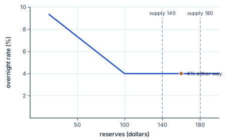
The same reserve injection can have different interest-rate consequences in different regimes. When reserves are scarce enough that the supply intersects a downward portion of reserve demand, adding supply can lower the clearing overnight rate. When supply lies on a sufficiently flat portion associated with administered returns, adding more reserves can leave the relevant market rate approximately unchanged. The diagram's regime is part of the answer, not an optional annotation.
Another way: steps
Identify the bank asset and central-bank liability involved. State whether reserves are limited or ample. Apply the supplied rate rule or reserve-demand relationship. Then trace the real-rate and expenditure links with their inflation-expectations, credit, and aggregate-supply assumptions.
Consider a fictional limited-reserve market with reserve demand R = 160 - 20i, where R is reserve dollars and i is the overnight nominal annual interest rate in percentage points. With supplied reserves of eighty dollars, equilibrium satisfies 80 = 160 - 20i, giving four percent. A purchase that adds twenty reserve dollars shifts the vertical supply to one hundred and produces a three-percent rate in this specified range.
The rate falls because banks need a smaller incentive to economize on scarce balances when more are supplied, given the downward demand relationship. This is a movement along reserve demand following a supply change. A higher demand for settlement balances would instead shift demand. The rate implications of simultaneous demand and supply changes require solving both changes rather than mechanically treating every purchase as a fixed rate reduction.
This reserve-market horizontal axis is bank balances at the central bank. It is not the household money-demand diagram's broad money stock and is not the annual funds flow used in loanable-funds analysis. The diagrams may interact in a larger model, but a label such as dollars alone is insufficient to identify which market is being solved. State the holder, issuer, and stock or flow nature of the quantity.
An open-market sale reverses the reserve-supply effect when its payment drains balances. In this limited-reserve model, fewer supplied reserves raise the rate along the given demand schedule. That conclusion requires remaining on the relevant downward portion and holding demand fixed. Changes in other facilities, expectations, regulations, or liquidity conditions could alter the relationship. The simple equation is a declared comparison, not a description of every central bank at every date.
The central bank can also respond to an increase in reserve demand by supplying enough balances to preserve a rate target. In that case, observing a larger reserve quantity alongside an unchanged rate does not show that policy became more expansionary. The quantity can be accommodating a change in demand. Distinguish a deliberate change in the targeted stance from operational actions that maintain it.
The figure shows why more reserves leave the rate unchanged: on the flat part of the demand curve, supply can move without moving the rate.
In an ample-reserves framework, the central bank supplies enough balances that small ordinary changes in their quantity have limited influence on the overnight rate. It uses administered rates to guide market rates. The Federal Reserve's interest on reserve balances provides banks with a return available on their reserve holdings. This return influences the terms on which banks are willing to lend or invest in other short-term instruments.
Not every participant has access to the same facility, and arbitrage can face balance-sheet costs, credit concerns, and other frictions. Therefore interest on reserves should not be described as a perfect mathematical floor under every market transaction. The overnight reverse repurchase facility offers an alternative to a broader eligible set of counterparties and helps support rate control. Its institutional role is distinct from customer deposits and from a compulsory reserve ratio.
For a fictional exercise, suppose the case explicitly gives the rule i = a whenever reserve balances are at least one hundred dollars, where a is an administered nominal rate. If reserves increase from 140 to 180 with a fixed at four percent, the model's market rate remains four percent. If a instead falls to three percent while reserves remain ample, the model's market rate falls to three percent. This exact equality is a simplifying exercise rule, not a claim of frictionless real-world implementation.
The threshold matters. A sufficiently large reserve drain could move the system outside the ample region and make quantity conditions influential again. A learner should not extend the flat rule below its stated domain. Likewise, the central bank may buy assets for purposes involving market functioning or longer-term yields as well as reserve supply. The effect must be tied to the mechanism the case actually specifies.
Modern bank lending is constrained by creditworthiness, profitability, capital, liquidity, regulation, and funding conditions. It is not governed by a universal fixed reserve multiplier. Changing an administered return alters opportunity costs and financial conditions; it does not force every additional reserve dollar into a prescribed number of new loans. A zero required reserve ratio does not imply unlimited safe or profitable credit creation.
Operational details can change over time. The Federal Reserve's published framework and interest-on-reserve-balances explanations support the distinction taught here, while all numerical rates and thresholds in this lesson are fictional. Institutional statements should be checked against current primary sources before being used to describe a later policy episode. The assessed task is to apply a clearly specified regime, not to memorize today's policy setting.
A lower nominal policy rate can lower other borrowing rates, but pass-through need not be immediate or complete. Different maturities, credit risks, lending standards, and expectations influence the rates households and firms face. A decline in the overnight rate does not guarantee that every risky borrower receives a cheaper loan. When a problem stipulates full pass-through to a relevant rate, use that assumption and identify it.
Expected inflation is essential to the expected real borrowing cost. Under a stated percentage-point approximation, the expected real rate is the nominal rate minus expected inflation. If the nominal rate falls from six to four percent while expected inflation stays at two percent, the approximate real rate falls from four to two percent. If expected inflation also falls by two percentage points, the same nominal reduction leaves that approximate real rate unchanged.
The exact purchasing-power formula divides the gross nominal return by the expected price-level growth factor and subtracts one. The subtraction formula is an approximation and should be labeled when used. A case that asks for exact arithmetic must use the ratio. Mixing an exact answer from one scenario with an approximate answer from another creates an artificial difference unrelated to policy transmission.
With an investment schedule I = 120 - 10r, a real rate decline from four to two raises desired investment from eighty to one hundred dollars per period. An aggregate-demand response then depends on spending propagation, exchange-rate channels, and other offsets. A fixed-price multiplier could amplify the initial investment change if its assumptions hold. An upward-sloping short-run aggregate supply curve divides a demand increase between output and the price level.
Policy effects occur with uncertain lags, and decision makers act on incomplete, revisable information. A supply disruption can raise inflation while reducing output, so a demand adjustment can involve competing stabilization objectives. Monetary policy does not directly manufacture the disrupted input or permanently increase productive capacity through a simple movement in aggregate demand. The mechanism analysis therefore cannot alone establish a universally best policy action.
Expectations may change before a scheduled action if markets anticipate it. Conversely, an unexpected announcement can affect longer-term conditions even before a balance-sheet transaction occurs. This observation does not mean every announcement has a predictable size or direction of effect. It means the relevant counterfactual includes what was already expected. A sound comparison states what is held fixed and distinguishes the instrument, intermediate rates, spending response, and final macroeconomic outcome.
A fictional central bank purchases forty dollars of securities from a commercial bank. Before the transaction, the bank holds 140 reserve dollars and eighty dollars of securities. The purchase raises its reserves to 180 and reduces its securities to forty. Its total assets are unchanged by this equal-value swap, and its customer deposits do not change merely because this bank sold its own securities.
The case states that reserves are ample whenever they are at least one hundred dollars and that the overnight rate equals the administered rate within this region. The administered rate remains four percent. A headline predicts that the purchase must lower the overnight rate to three percent because reserve supply increased. That prediction applies the wrong regime. Under the supplied ample-reserve rule, the rate stays four percent.
A separate announced action reduces the administered rate to three percent while reserves remain at 180. Under the same rule, the overnight rate now becomes three percent. The instrument that changes the modeled rate is the administered return, while the purchase changed the composition of the bank's assets. The distinction makes the balance-sheet explanation and the rate explanation consistent.
This result does not establish that asset purchases can never affect any yield. A broader model might include duration, portfolio-balance, expectations, or market-functioning channels that influence other financial conditions. Those channels are not part of this numerical case. The responsible conclusion is that the stated overnight rate does not move with this reserve addition in the declared ample region, and that further claims require additional mechanisms and evidence.
Reserve balances and customer deposits are different liabilities of different issuers. An asset swap with a bank need not create a customer deposit. Quantity changes can matter in a limited-reserve regime while administered rates guide an ample-reserve regime. A nominal rate reduction changes expected real costs only after accounting for inflation expectations, and a spending response still requires behavioral assumptions.
Record the reserve-demand equation.
R=160-20i, with i in annual percentage points.
The rate units determine how the coefficient is used.
Record the supplied reserve stock.
R supply=80 reserve dollars.
This is a bank settlement-balance stock rather than an annual saving flow.
Equate desired and supplied balances.
80=160-20i.
A clearing rate reconciles the given demand with the available stock.
Solve the initial overnight rate.
20i=80, so i=4%.
The supplied demand relation is downward in this limited-reserve range.
Check a twenty-dollar injection.
100=160-20i gives i=3%.
Greater supply lowers the rate along the unchanged demand relationship.
Identify the rule's domain.
For R≥100, the exercise sets i=a.
The flat relation applies only where reserve balances are ample.
Check the starting reserve quantity.
R=140 is above the threshold.
The administered-rate rule is applicable to the initial state.
Apply the stated administered rate.
a=4% gives i=4%.
The problem explicitly supplies exact pass-through in this simplified framework.
Add reserves while preserving the instrument.
R=180 and a=4% still give i=4%.
The quantity change remains inside the ample region.
Change the administered return separately.
R=180 and a=3% give i=3%.
This comparison isolates the instrument that changes the rate under the given rule.
State the nominal borrowing-rate change.
The relevant nominal annual rate falls from 6% to 4%.
The case assumes full pass-through from the policy instrument to this borrowing rate.
Hold expected inflation fixed.
Expected annual inflation remains 2%.
A nominal change alone does not establish the real-cost change.
Use the stipulated real-rate approximation.
Approximate r falls from 6-2=4% to 4-2=2%.
Subtraction is the supplied approximation rather than the exact gross-return ratio.
Evaluate the initial investment schedule.
I=120-10×4=80 dollars per period.
The behavioral equation relates investment to the expected real rate.
Evaluate the new investment schedule.
I=120-10×2=100 dollars per period.
Other profitability and financing conditions are held fixed.
Limit the output conclusion.
Desired investment rises twenty; the final output effect needs an aggregate model.
Capacity, price adjustment, and other spending responses determine how this initial change propagates.
Identify the central bank's seller.
The seller is a commercial bank holding its own securities.
A purchase from a nonbank would involve a different deposit entry.
Record equal asset changes at the bank.
Reserves rise forty and securities fall forty dollars.
Settlement exchanges one bank asset for another at the stipulated value.
Check the bank's liability side.
A fictional limited-reserve market has R=180-20i, where R is reserve dollars and i is the nominal annual rate in percentage points. Compute the clearing rate for reserve supplies of eighty and one hundred dollars.
| Rate percent | |
|---|---|
| R=80 | |
| R=100 |
A fictional limited-reserve market has R=200-25i, where i is annual nominal percentage points. Reserves initially equal one hundred dollars and then increase by twenty-five. Complete the initial rate, final rate, and rate change.
Solve the initial reserve-market intersection.
Initial nominal rate=initial percent.
Set the supplied stock equal to the given reserve demand.
Solve the intersection after the injection.
Final nominal rate=final percent.
Demand remains unchanged while the supplied reserve quantity increases.
Subtract the initial rate from the final rate.
Rate change=change percentage points.
A rate difference is reported in percentage points rather than a percent growth rate.
In a fictional ample-reserve regime, the overnight nominal rate equals four percent whenever reserves are at least one hundred dollars. Plot the rate at reserve stocks120,160,200. Reserve dollars are horizontal; rate percent is vertical.
Plot your answer on the grid:
A fictional borrowing rate falls from six to four percent annually. Use the approximation r=i-expected inflation. Compare case A, where expected inflation stays two percent, with case B, where it falls from two to zero percent. Give each case's new approximate real rate and its percentage-point change from the initial rate.
| New real rate percent | Change percentage points | |
|---|---|---|
| A | ||
| B |
Construct the stipulated transmission chain. Reserves remain ample, the administered rate falls, full pass-through lowers the relevant borrowing rate, expected inflation stays fixed, and investment falls with the expected real rate. Each node states a conditional link supplied by the case.
This task has no paper form; do it on a device.
A fictional commercial bank owns reserves60 and securities90 dollars; deposits are130 and equity20 dollars. The central bank purchases thirty dollars of that bank's own securities at their recorded value. No other transaction occurs. Complete the bank's new balance sheet.
| Dollars | |
|---|---|
| Reserves | |
| Securities | |
| Deposits | |
| Equity |
Lesson test: one question per skill, one attempt each, no hints. Your answers are checked when you submit.
A fictional ample-reserve rule is i=a for reserves R≥100 dollars. Initially R=140 and administered rate a=5%. First reserves rise to180 with a unchanged. Then a falls to3% while R remains180. Assuming full borrowing-rate pass-through, fixed expected inflation1%, and the approximation r=i-expected inflation, give the market rate after each action, the final real rate, and final investment from I=100-10r dollars per period.
| Value | |
|---|---|
| Rate after reserves rise percent | |
| Rate after administered cut percent | |
| Final approximate real rate percent | |
| Final investment dollars per period |
You can identify which policy instrument moves the rate in a declared regime and which assumptions connect it to spending. Next, examine how inflation expectations change stabilization relationships.
13. Separate an asset swap from deposit creation, step 3
Customer deposits and equity remain unchanged in this isolated transaction.
No customer sold an asset or received a new deposit in this case.