Back to the on-screen lesson ·
Solve and compare aggregate equilibria under explicitly specified demand and supply changes.
Paper packet. Every task here also exists on screen, where it is checked automatically; answers written on paper are not assessed by Nydus. When you are back at a device, enter your answers there.
Construct equilibrium price-output pairs, plot supplied-model intersections, compute output gaps, and distinguish demand, supply, and combined-shock explanations while identifying missing dynamic assumptions.
You can distinguish movements from shifts on AD and SRAS and track a separate potential-output benchmark. Now solve the output-price pair that lies on both curves. A result belongs to the supplied equations and adjustment assumptions, not to a forecast about an actual economy.
| Term | What it means |
|---|---|
| Short-run equilibrium | A price-output pair consistent with the supplied aggregate-demand and short-run aggregate-supply relationships. |
| Recessionary gap | Actual equilibrium output below the stated potential benchmark. |
| Inflationary gap | Actual equilibrium output above the stated potential benchmark in the introductory model. |
| Demand shock | A change in a nonprice determinant shifting aggregate demand. |
| Adverse supply shock | A cost or productive-condition change reducing short-run output supplied at a given price level. |
| Comparative statics | Comparison of equilibria before and after a specified change, without a complete time path. |
Suppose a fictional model has AD given by P = 200 - Y and SRAS by P = 40 + Y. Y is real output in base-year dollars and P is a price index. At their intersection, both equations must describe the same price, so 200 - Y = 40 + Y. Rearranging gives 160 = 2Y and Y = eighty. Substituting into either equation gives P = 120.
An algebraic solution must also lie inside the domain where the relationships are meant to apply. If solving a supplied system produced negative real output or a price index outside its stated range, report the inconsistency instead of interpreting the number as an economic equilibrium. The examples here choose positive intersections within the displayed domains. This domain check complements substitution: satisfying two formulas is insufficient when the model restricts the values those formulas represent.
Checking both equations is important. AD gives 200 - 80 = 120 and SRAS gives 40 + 80 = 120. A pair that satisfies only one curve is a point on that schedule, not the model's equilibrium. The equations and the graph are two representations of the same simultaneous conditions. Plotting the pair uses the coordinate (80,120), with output horizontal.
If potential output is one hundred, this equilibrium has an output gap of negative twenty percent. The gap does not alter the algebraic fact that AD and SRAS intersect at eighty. It adds a comparison with a longer-run benchmark. Short-run equilibrium and full-employment equilibrium are therefore distinct concepts: plans can be mutually consistent in the short-run model while output remains below potential.
Another way: steps
Write the AD and SRAS equations in compatible units. Equate their price expressions and solve for output. Substitute into both equations to verify the price. Only then compare output with the stated potential benchmark and interpret the specified shock.
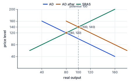
The figure draws this case: the new crossing lies on the unchanged supply curve, at higher output and a higher price level.
Starting from P = 200 - Y and P = 40 + Y, suppose a nonprice spending change shifts AD to P = 240 - Y while SRAS remains fixed. The new equation is 240 - Y = 40 + Y, giving Y = one hundred and P = 140. Both output and the price level rise in this supplied upward-SRAS model. The demand shift is not identical to the output increase because some adjustment occurs through prices.
The new equilibrium lies on the unchanged SRAS curve. Firms move along that relationship as the equilibrium price changes; SRAS has not shifted merely because its equilibrium quantity changed. This distinction is a useful graphing check. One event can shift AD and create movement along SRAS at the same time, without requiring both curves to move.
The size of the output response depends on the slopes. With a flatter SRAS over the relevant range, a similar demand shift can produce more output adjustment and less price adjustment. With a steeper SRAS, more of the adjustment appears in prices. A vertical supply benchmark implies no output response to the demand shift within that long-run comparison. The direction and magnitude are therefore conditional on the production side of the model.
If potential remains one hundred, the original twenty-percent recessionary gap closes in the example. That does not establish that the spending change was costless or optimal. The model records an output and price comparison, while policy evaluation might also require distribution, financing, implementation lags, uncertainty, and future effects. A graph intersection cannot decide value judgments that the model has not encoded.
If the demand shift were larger, equilibrium could exceed potential in the short run. The introductory label inflationary gap indicates above-potential output and possible upward cost or price pressure during adjustment. It does not specify an inflation rate from the gap percentage alone. A twenty-percent output gap is not automatically twenty-percent inflation; those are different measured changes linked only through an additional model.
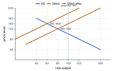
The figure draws this case: output falls to sixty while the price level rises to 140.
Now return to the initial AD equation P = 200 - Y, but shift SRAS from P = 40 + Y to P = 80 + Y. Equating gives 200 - Y = 80 + Y, so Y = sixty and P = 140. Output falls while the price level rises. This differs from the positive-demand-shock case, where both rose. Observing a higher price level alone cannot distinguish the two mechanisms.
The combination of weaker activity and rising prices is often discussed using the term stagflation, although an actual diagnosis involves changes over time and several indicators. Our one-step comparison establishes lower real output and a higher price level under the specified cost shock. It does not imply that every inflation episode has that cause or that the shock's effects will persist indefinitely.
If potential remains one hundred because the cost shock is temporary, the new gap is negative forty percent. If the shock also destroys sustainable capacity, potential must be revised separately before computing the gap. The same observed output of sixty could imply different gaps under different capacity estimates. This is why a supply-shock question must state whether productive resources and technology are unchanged.
A demand expansion in response to an adverse supply shift can partly restore output while raising prices further in the simple model. A demand contraction can restrain the price level while reducing output further. This conditional tradeoff is a model result, not a recommendation for either response. An evaluation would depend on the shock's persistence, expectations, objectives, available supply responses, and uncertainty about the relevant relationships.
The model can also describe a favorable supply shock. A lower SRAS intercept with AD fixed raises equilibrium output and lowers the price level under the same slopes. If productivity also raises potential, the new gap requires the updated benchmark. Do not infer the gap's direction from the output direction alone when both actual output and potential change.
Suppose AD and SRAS both shift upward by twenty index points from the initial equations. The new relationships are P = 220 - Y and P = 60 + Y. The intersection remains Y = eighty, while P rises to 140. The demand shift raises output, the cost shift lowers it, and their stated magnitudes exactly offset in this linear model. An unchanged output observation can conceal substantial changes in the underlying relationships.
If only the directions of those shifts were given, the output effect would be ambiguous. Prices would rise in the standard diagram because both changes put upward pressure on the equilibrium price, but output could rise, fall, or remain unchanged depending on the relative shifts and slopes. A rigorous answer separates the determinate and indeterminate dimensions instead of forcing one unqualified directional conclusion.
Comparative statics does not show the actual path between equilibria. The economy might move gradually, overshoot, or experience additional shocks. The lines identify internally consistent endpoints under the assumptions. To describe timing, unemployment dynamics, inventories, or expectation formation along the route, a dynamic model would be needed. Do not label the straight arrow between two intersections as an empirically observed transition unless such data are supplied.
For a long-run adjustment comparison, hold AD at P = 200 - Y and potential at one hundred. A long-run point on AD at potential has P = one hundred. If SRAS takes the form P = a + Y, its intercept must become zero to pass through that point. This algebra identifies the supply relationship consistent with return to potential. It does not prove that wages will actually adjust at a particular speed or that the assumed potential remains unchanged throughout a recession.
An alternative model could hold nominal costs rigid for longer, allow expectations to move differently, or permit potential to decline through lost investment and labor attachment. These assumptions can generate different paths and endpoints. The course assesses the logic within each stated case and the assumption responsible for the difference, not allegiance to a school of thought.
Good model comparison preserves a common baseline and changes one condition at a time where possible. If the demand shift, supply slope, and potential benchmark all change, list them separately and solve the new system before attributing the difference to a single cause. This discipline prevents a graph from becoming a picture chosen to confirm a preferred story.
A fictional economy starts at the intersection of P = 200 - Y and P = 40 + Y, giving Y = eighty and P = 120. Two analysts present different counterfactuals. Analyst A shifts demand to P = 240 - Y and leaves supply unchanged. Analyst B leaves demand unchanged but shifts supply to P = 80 + Y. Both report a new price index of 140.
Analyst A's new output is one hundred. Analyst B's new output is sixty. Their price results agree, but their mechanisms and output implications differ. A price observation alone cannot select between these explanations. Evidence about spending determinants, input costs, production, and the timing of the events would be needed to assess which model better represents an actual episode.
With potential fixed at one hundred, A's output gap is zero and B's is negative forty percent. These gaps are conditional on the common capacity assumption. If B's event includes permanent capital destruction, using the original potential without examination could misstate the gap. The analyst should say whether the shock changes only current costs or also sustainable productive capacity.
A review should reproduce the equations, solve both intersections, and identify the changed assumption before comparing policy implications. It should not choose a model because the outcome sounds preferable. Nor should it treat the shared price index as evidence that the two analyzes are equivalent. The example illustrates how a complete equilibrium comparison contains more information than one headline variable.
An equilibrium pair must satisfy both curves. A demand shift can cause movement along unchanged SRAS. The same price change can accompany opposite output changes under different shocks. An output-gap percentage is not an inflation rate. Comparative statics identifies endpoints, while adjustment speed and paths need additional assumptions.
Write the two price expressions.
AD: P=200-Y; SRAS: P=40+Y.
At equilibrium they refer to the same price and output.
Equate and collect output terms.
200-Y=40+Y; 160=2Y.
Simultaneous consistency eliminates the price variable.
Solve for real output.
Y=80 base-year dollars.
Dividing by the combined slope coefficient gives the intersection's horizontal coordinate.
Substitute into both curves.
AD: 200-80=120; SRAS: 40+80=120.
Agreement verifies the price coordinate.
Compare with supplied potential.
Potential 100 gives (80-100)/100=-20%.
The capacity comparison follows after finding short-run equilibrium.
Replace only the demand equation.
New AD: P=240-Y.
The shock changes a nonprice spending determinant.
Keep the supply relationship fixed.
SRAS remains P=40+Y.
Costs and expectations are unchanged in this counterfactual.
Solve the new simultaneous conditions.
240-Y=40+Y; Y=100.
The intersection changes in both output and price.
Verify the new price.
240-100=140 and 40+100=140.
The new point lies on the unchanged SRAS curve.
Interpret the fixed-capacity comparison.
At potential 100, the output gap is zero.
Closing this gap is a conditional result, not a complete policy evaluation.
Use the common starting equilibrium.
Y=80 and P=120.
A shared baseline makes the counterfactuals comparable.
Solve the demand-shift case.
AD P=240-Y with original SRAS gives Y=100,P=140.
Higher spending raises both coordinates under the stated slopes.
Solve the cost-shift case.
Original AD with SRAS P=80+Y gives Y=60,P=140.
Higher costs lower output while raising price.
Compare the common observed variable.
Both price indexes are 140.
A matching price result does not identify the same underlying cause.
Compare output and gaps.
Outputs 100 and 60; at potential 100, gaps 0% and -40%.
The production consequences differ even though prices match.
Identify evidence needed beyond the model.
Check spending changes, cost changes, output, and capacity assumptions.
Selecting a real-world explanation requires evidence about the mechanisms rather than preference for an outcome.
Write the two shifted equations.
AD P=220-Y; SRAS P=60+Y.
Both intercepts rose by twenty from the original model.
Solve the new intersection.
220-Y=60+Y; Y=80,P=140.
The equal shifts offset in the output equation.
Interpret both coordinates.
A fictional AD–AS model uses P=180-Y and P=20+Y. Real output Y is in base-year dollars. Potential is one hundred. Compute equilibrium output, price index, and output-gap percent.
| Value | |
|---|---|
| Equilibrium Y | |
| Equilibrium P | |
| Output gap percent |
A fictional model has AD P=210-Y, SRAS P=30+Y, and potential output one hundred base-year dollars. Complete the simultaneous solution and gap.
Equate demand and supply prices and solve output.
Equilibrium Y=output.
The intersection requires both price expressions to agree.
Substitute the output into either equation.
Equilibrium P=price.
Both equations must give the same result.
Compare output with the stated capacity.
Output gap=gap percent.
Use potential output as the denominator.
Plot only the initial and new equilibrium points for two fictional models. Initially AD is P=160-Y and SRAS P=40+Y. Later AD is P=200-Y with unchanged SRAS. Horizontal Y is real output in base-year dollars; vertical P is the price index.
Plot your answer on the grid:
A fictional economy has AD P=240-Y. Initial SRAS is P=40+Y; after a temporary cost shock it is P=80+Y. Potential stays one hundred. Compute both equilibria and their output gaps.
| Y | P | Gap percent | |
|---|---|---|---|
| Initial | |||
| After cost shock |
Construct the reasoning explaining why a higher price level alone does not identify an aggregate shock. The cases use ordinary upward SRAS and downward AD.
This task has no paper form; do it on a device.
A fictional port economy initially has AD P=200-Y and SRAS P=40+Y. New export orders shift AD to P=230-Y while a shipping-cost shock shifts SRAS to P=70+Y. Potential is unchanged. Compute original and new equilibrium output and price.
| Y | P | |
|---|---|---|
| Original | ||
| Both shocks |
Lesson test: one question per skill, one attempt each, no hints. Your answers are checked when you submit.
A fictional model starts with AD P=260-Y and SRAS P=60+Y, with potential output one hundred. A cost shock changes only SRAS to P=100+Y. Compute initial Y and P, new Y and P, and the new gap percent. All output is in base-year dollars.
| Value | |
|---|---|
| Initial Y | |
| Initial P | |
| New Y | |
| New P | |
| New gap percent |
You can solve both curves together and explain why one price observation cannot identify a shock. Next, derive a spending multiplier only under the assumptions that make repeated expenditure rounds valid.
13. An equal pair of opposite output pressures, step 3
Output is unchanged at eighty while price rises from 120 to 140.
An unchanged aggregate can conceal opposing underlying shocks.