Distinguish shifts from movements and preserve ambiguous predictions
Paper packet. Every task here also exists on screen, where it is checked automatically; answers written on paper are not assessed by Nydus. When you are back at a device, enter your answers there.
1. What you will learn
Distinguish shifts from movements and preserve ambiguous predictions
2. Starting point
At equilibrium, planned purchases equal offers at a common price. An own-price change moves along fixed schedules; other influences can change the schedules themselves.
3. Words for this lesson
Term
What it means
Demand shift
A change in quantity demanded at a given own price because another influence changed.
Supply shift
A change in quantity supplied at a given own price because another influence changed.
Normal good
A good whose demand rises with income over the specified range, other things equal.
Substitute
An alternative good whose price increase can raise demand for the good being studied.
Complement
A good used with another, whose price increase can reduce demand for that other good.
Ambiguous prediction
A direction that cannot be determined without more information about the relative changes.
4. A shift changes a conditional relationship
A demand schedule says what buyers plan at different own prices while other influences are held fixed. If those other influences change, buyers may plan a different quantity even at the same own price. That is a shift in demand. The key comparison is between old and new quantities at a common price, not merely between two observed sales totals.
Suppose buyers previously demanded ten notebooks at three tokens and now demand fourteen at that same price after more buyers enter the market. The four-unit increase is evidence of a demand shift in the supplied model. If the notebook price instead fell and the original schedule already predicted fourteen at the lower price, that would be movement along demand. Similar quantity changes can have different causes.
A supply shift is defined in the same conditional way. If cheaper paper enables sellers to offer more notebooks at every listed notebook price, supply shifts outward. At a common price of three, an increase from ten offered to fourteen is a shift if the cause is the changed input condition. If notebook price rose along the old supply schedule, the resulting quantity increase would instead be movement along supply.
Always identify the market before identifying the cause. The price of paper is an input price for notebook producers, but it is the own price in the paper market. One event can play different roles in different models. A statement such as 'price changed, so there is movement' is incomplete until we know which price and which market are being analyzed.
Another way: Identify demand influences without assuming their direction
Changes in the number of buyers, preferences, income, expectations and related-good prices can affect demand. The direction needs information about the relationship. More buyers with positive planned purchases generally increase market demand when the original buyers' behavior stays fixed. A change in preference toward the good also increases demand under the stated comparison.
Income requires care. For a normal good over a specified range, higher income raises demand, other things equal. For an inferior good over that range, higher income reduces demand as buyers choose alternatives. These labels describe a response to income, not product quality or a judgment about the people who buy it. A question must supply or justify the relevant classification before asking for a direction.
Related goods also require an explicit relationship. If tea and coffee are substitutes in the case, a higher coffee price can increase demand for tea. If printers and compatible ink are complements, a higher printer price can reduce demand for ink. These are changes in another good's price, so they shift the focal good's demand rather than move along it.
Expectations can alter timing. A buyer expecting a future price increase may bring a purchase forward, but the response depends on storage, urgency, resources and the credibility of the expectation. Do not turn a possible mechanism into a universal guarantee. In exercises, use the stated assumptions. In an actual market, the direction and size of the response require evidence about the participants and alternatives.
Another way: Identify supply influences and the relevant horizon
Input costs, technology, productive capacity, the number of sellers and some taxes or subsidies can change supply. A reduction in the cost of producing each unit can make greater quantities attractive at each output price in a competitive model. Improved technology can have a similar effect when it reduces resource requirements. An interruption that removes usable capacity can reduce offers at the same price.
The event must affect the market under study during its stated period. A new factory planned for next year may not increase this afternoon's deliverable supply. A temporary shipping disruption may reduce available deliveries even if the factories' technical capacity is unchanged. Economic explanations need timing and a mechanism, not just a favorable or unfavorable word.
Some events affect more than one curve. A storm can damage productive facilities and also change what households want to buy. A publicity campaign might attract consumers and encourage sellers to enter. If the exercise states that only supply changes, hold demand fixed for that model. If it gives evidence of changes on both sides, analyze both rather than force the event into one category.
A seller's expectations can also affect current offers when goods can be stored or production can be delayed. The direction is not automatic for every product. Perishable goods, services tied to a date and durable inventories differ. The introductory cases specify simple shifts so that the reasoning can be checked, while the explanation should acknowledge which assumptions make that simplification appropriate.
Another way: Trace one shift through both sides of the market
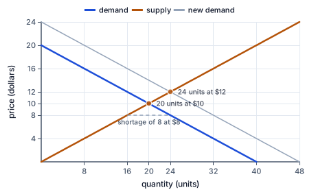
Price in dollars against quantity in units. Demand Qd = 40 - 2P falls and supply Qs = 2P rises; they cross at 20 units and 10 dollars. At 8 dollars buyers want 24 and sellers offer 16, a shortage of 8. Demand shifted out to Qd = 48 - 2P crosses the same supply curve at 24 units and 12 dollars.
The figure shows one shift traced through: demand moves out while supply stays put, and the crossing moves up and to the right along the unchanged supply curve.
With an upward supply curve fixed, an outward demand shift normally raises equilibrium price and quantity in the introductory model. At the old price, buyers now want more than sellers offer. A price increase can reduce quantity demanded along the new demand curve and raise quantity supplied along the unchanged supply curve until the plans agree.
Notice the two different descriptions in that chain. Demand shifted because a non-price influence changed. Supply did not need to shift; sellers changed quantity supplied in response to the new own price. Saying that both curves shift whenever both quantities change confuses the cause with the resulting movement. At equilibrium the traded quantity belongs to both sides, but that does not mean both relationships changed.
With demand fixed, an outward supply shift normally lowers equilibrium price and raises equilibrium quantity. At the old price, offers exceed planned purchases. A lower price encourages purchases along unchanged demand while reducing offers along the new supply schedule relative to what sellers would offer at the old price. The final quantity can still exceed its original equilibrium value.
Reverse shifts reverse these standard directions under the same shapes and assumptions. Reduced demand lowers price and quantity; reduced supply raises price and lowers quantity. These are conditional comparative results, not a promise about the speed or path of adjustment. A table or set of equations can establish exact before-and-after equilibria without proving that the real market moves smoothly between them.
Another way: Two simultaneous shifts can leave one result unresolved
Suppose both demand and supply increase. Each shift, considered on its own with ordinary slopes, raises equilibrium quantity. Their effects on price oppose each other: stronger demand pushes price upward, while greater supply pushes it downward. Quantity rises, but price may rise, fall or stay unchanged depending on the relative changes.
This ambiguity is a correct result, not a failure to finish. Without magnitudes or complete new schedules, there is not enough information to choose one price direction. Guessing that the more dramatic story must dominate is not a valid calculation. If the case supplies old and new tables, solve them directly; if it supplies only directions, report only the directions supported by the assumptions.
If demand rises while supply falls, both changes push price upward, while their quantity effects oppose. Price rises under the standard model, and the quantity direction is unresolved without further information. If demand falls while supply rises, price falls and quantity is ambiguous. If both fall, quantity falls while price is ambiguous. Reason through the two separate effects instead of memorizing an unexplained grid.
These results assume the familiar downward demand and upward supply relationships with suitable intersections. Unusual shapes, capacity corners or discrete quantities can require a more careful analysis. The exercises state the standard model when they ask for qualitative arrows. A responsible explanation keeps those conditions visible and does not extend a simple diagram beyond its defined range.
Another way: Use counterfactual comparisons rather than loose stories
A before-and-after observation can be consistent with several causes. Higher price and quantity could result from an outward demand shift along fixed supply, but other combinations of changes might produce the same observation. The outcome alone does not uniquely identify the cause. A causal explanation needs information about what changed and what would have happened otherwise.
An explicit table helps make the counterfactual clear. Keep the old supply schedule, replace only demand with the new schedule, and find the new equality. This answers what the supplied model predicts if demand alone changes. Replacing both schedules answers a different question. Label each scenario so that quantities from different counterfactual worlds are not accidentally combined.
When recording changes, compute new minus old for both price and quantity. A positive difference indicates an increase; a negative one a decrease; zero means unchanged. Report units separately: a price difference is tokens per unit, while a quantity difference is units per period. These differences summarize the comparison but do not measure welfare or the desirability of the event.
Finally, distinguish uncertainty about the model from ambiguity inside the model. We may know the exact shifts in a classroom table and calculate a precise result, while still being uncertain whether that table represents a real market. Or we may accept the model shapes but lack shift magnitudes, leaving a direction ambiguous. Naming the missing information makes the answer more useful than an unsupported confident prediction.
5. A repair market after a community event
A fictional repair market initially clears at five tokens per repair and twelve repairs per week. A community event encourages more people to repair items. The supplied new demand schedule, combined with unchanged supply, clears at seven tokens and sixteen repairs. The model therefore predicts a price increase of two and a quantity increase of four when demand alone changes.
At the same time, a new tool could reduce the time required for each repair. If the case introduces that tool, supply may also increase. Demand and supply then both move outward. Under the standard slopes, the quantity direction remains upward, but the price direction is no longer determined by the demand story alone. The tool's supply effect could offset some, all or more than all of the upward price effect.
Suppose the complete revised schedules instead clear at four tokens and twenty repairs. With those additional numbers, price falls by one and quantity rises by eight compared with the original equilibrium. This does not contradict the earlier ambiguity. It supplies the magnitudes that were previously missing and selects one of the outcomes the qualitative analysis allowed.
The organizer should not infer that every participant benefits from the lower price. Repairers may face different tool costs, and customers differ in access and needs. The market calculation identifies conditional price and quantity changes. Evaluating the program also requires information about costs, distribution and effects outside the transactions. Keeping those questions separate makes the model easier to audit and prevents a plausible story from becoming an unsupported policy conclusion.
6. A tempting mistake
An increase in equilibrium quantity does not imply both curves shifted. When two shifts have opposing effects on an outcome, direction alone cannot determine that outcome's net change.
7. An own-price change is movement
Identify the market.
Notebooks per week
The own price is the notebook price.
Read the fixed demand rows.
P=4: Q=6; P=2: Q=10
Other influences are unchanged.
State the event.
Notebook price falls from 4 to 2
Only own price changes here.
Read the response.
Quantity demanded rises by 4
The response is already on the old schedule.
Classify the change.
Movement along demand
No new demand relationship is needed.
8. Demand shifts while supply stays fixed
Read the old equilibrium.
P=3, Q=10
This is the baseline.
State the non-price event.
More buyers enter
The market demand schedule changes.
Hold the other side fixed.
Original supply remains
No supply shift is assumed.
Read the new equality.
P=5, Q=14
The new demand and old supply intersect here.
Describe both changes.
Price +2; quantity +4
Sellers move along fixed supply in response to the new price.
9. Both curves move outward
State the model shapes.
Downward demand, upward supply
These shapes support the standard directional comparison.
Isolate the demand effect.
P up, Q up
More demand raises both with supply fixed.
Isolate the supply effect.
P down, Q up
More supply lowers price and raises quantity with demand fixed.
Combine quantity effects.
Q up
Both point in the same direction.
Compare price effects.
Opposing directions
Their relative sizes have not been supplied.
Report the supported result.
Q rises; P ambiguous
Additional magnitudes are needed to resolve price.
10. Complete a before-and-after comparison
Read the old pair.
P=6,Q=10
Use the same price and quantity units throughout.
Read the new pair.
P=4,Q=15
The complete revised schedules supply this equilibrium.
Your turn: work this step out. Its working is at the end of the packet.
Compute signed changes.
11. Guided practice
Under the supplied old schedules, equilibrium is P=3 tokens and Q=12 units per week. Under the complete new schedules it is P=5, Q=16. Enter each signed change as new minus old.
Your result
Price change
Quantity change
12. Guided practice
An old equilibrium quantity is eleven and the revised quantity is eighteen units per week. Fill the signed quantity change.
Keep the comparison order.
New minus old
This convention determines the sign.
Subtract the old quantity.
18-11=dq
Both quantities share the same weekly unit.
Check the reverse account.
11+dq=18
The signed change reconstructs the new quantity.
13. Guided practice
For the notebook market, match the stated event to its direct model change. Other influences stay fixed.
Movement along a fixed schedule
Demand shift
Supply shift
Notebook own price changes on the existing schedule
More buyers demand notebooks at every listed price
Cheaper paper raises notebook offers at every listed price
14. Practice
At a fixed notebook price of four tokens, old planned demand was ten and new planned demand is fourteen after more buyers enter; supply stays twelve. The new demand schedule also gives eight at a price of six. Enter the same-price demand change and supply change. Then enter the demand-quantity change when own price moves from four to six on the NEW schedule. Finally code that last event: 1 means movement along a fixed schedule, 2 means a new shift. All quantities are notebooks per week.
Demand shift at the common price: b0
Supply change at the common price: b1
Quantity change on new demand: b2
Last event code: b3
15. Practice
Under the supplied old schedules, equilibrium is P=4 tokens and Q=12 units per week. Under the complete new schedules it is P=4, Q=20. Enter each signed change as new minus old.
Your result
Price change
Quantity change
16. Somewhere new
Under the supplied old schedules, equilibrium is P=5 tokens and Q=12 units per week. Under the complete new schedules it is P=4, Q=20. Enter each signed change as new minus old.
Your result
Price change
Quantity change
17. Lesson test
Lesson test: one question per skill, one attempt each, no hints. Your answers are checked when you submit.
18. Test question
Use the standard downward demand and upward supply model. Demand increases and supply decreases, with neither shift's size given. Code each direction using 1 = increase, -1 = decrease, 0 = necessarily unchanged, 9 = ambiguous without magnitudes. Enter price and quantity directions.
Price direction: b0
Quantity direction: b1
19. What you can do now
Explain how to distinguish shifts from movements and preserve ambiguous predictions. Show a fresh example and check its result.
Working for the steps left to you
10. Complete a before-and-after comparison, step 3