Read and aggregate quantities demanded at a common price
Paper packet. Every task here also exists on screen, where it is checked automatically; answers written on paper are not assessed by Nydus. When you are back at a device, enter your answers there.
1. What you will learn
Read and aggregate quantities demanded at a common price
2. Starting point
Opportunity cost compares feasible alternatives. A buyer has a limited budget, and the price paid for one good affects what remains for other uses.
3. Words for this lesson
Term
What it means
Demand
The quantities buyers are willing and able to buy at different own prices under stated conditions.
Quantity demanded
The planned quantity at one specified price and under the stated conditions.
Schedule
A table pairing each price with the corresponding quantity.
Other things equal
An instruction to hold the other specified influences fixed during a comparison.
Market demand
The sum of individual quantities demanded at the same price in the same market and period.
Movement along demand
A change in quantity demanded caused by changing the good's own price on a fixed schedule.
4. Specify the market before counting
A demand schedule describes planned purchases at a series of possible prices. It needs a good, a unit, a group of buyers and a period. 'Six drinks' leaves many questions open. 'Six identical bottles per afternoon from these two buyers when each bottle costs two tokens' supplies the information needed for a model. The tokens are a fictional unit of payment, not a claim about a current currency or actual shop.
Willingness and ability both matter. Someone may want ten bottles but have resources for only two. A schedule should represent the quantities the person would choose and could purchase under its stated budget and conditions. It does not count every wish. Equally, having enough money does not imply wanting to spend all of it on the particular good. A person with a large budget might choose no bottles at all.
Consider a buyer whose schedule lists prices of one, two and three tokens, with quantities six, four and two bottles. These are alternative price scenarios for the same afternoon. Do not add the three quantities to claim twelve bottles are demanded that afternoon. Only one listed price scenario applies at a time. A row states a conditional plan, not a separate completed transaction.
Keep quality and unit size constant while comparing rows. A price of two tokens per small bottle cannot be compared directly with three tokens per large bottle as though only price changed. A different product, delivery condition or package might require a different schedule. Accurate arithmetic begins with a sufficiently precise description of the thing being counted.
Another way: Read a quantity at a given price
To use a supplied table, first find the stated price and then read the quantity in that same row. If price is three and the row reports two bottles, quantity demanded is two. Taking price from one row and quantity from another produces a combination the schedule does not contain. The table is a set of paired values, not two unrelated lists.
Demand names the whole schedule. Quantity demanded names one row's quantity. This distinction helps us describe a change precisely. If the bottle price falls from three to two while other influences stay fixed, quantity demanded rises from two to four on the same schedule. Saying that the entire demand schedule increased would imply a different kind of change, which we will examine later.
The schedule can contain zero. At a sufficiently high price a buyer may prefer to use the budget entirely elsewhere. Zero planned purchases does not show that the good has no possible usefulness, or that the buyer could never want it under different circumstances. It is a choice under the stated price, resources and preferences.
A table may list only several prices. Unless the case supplies an interpolation rule, do not invent the quantity at an unlisted price. Knowing the quantities at two and four tokens does not by itself establish the quantity at three. A straight connecting line would be an additional modeling assumption. In these exercises, each requested price is listed or an explicit rule supplies the missing information.
Another way: Why quantity may respond to price
For many goods over ordinary ranges, a lower own price leads buyers to plan more purchases, with other influences held fixed. One reason is substitution: the good becomes cheaper relative to alternatives. Another is purchasing power: a given budget can now buy more. These ideas explain why a downward relationship is a useful starting model rather than merely a pattern to memorize.
Suppose a snack becomes cheaper while the prices of all other lunch items remain unchanged. A buyer might substitute toward that snack, or keep buying the old quantity and use the money saved elsewhere. The schedule records the total planned response for the case. It does not require everyone to increase purchases by the same number or proportion.
The qualification about other influences is essential. A price decrease on the same day that the buyer loses all spending money need not produce more purchases. That observation combines changes in more than one influence. It does not isolate the own-price response described by the fixed schedule. We can analyze a simplified relationship without pretending that real events always change one thing at a time.
The downward pattern is not a definition that makes every other pattern logically impossible. More advanced economics examines special cases and the assumptions behind demand behavior. At this level, use the supplied schedule and its stated conditions. If the numbers differ from the usual pattern, read them accurately and question the model or evidence rather than silently rewriting them to fit a slogan.
Another way: Add buyers at a common price
Market demand combines quantities across buyers at the same price. Suppose at two tokens buyer A plans four bottles and buyer B plans three. Their combined quantity is seven bottles. If the price is three tokens and their quantities are two and one, combined quantity is three. Each market row is formed separately using a common own price and a common period.
Do not add the prices together. Both buyers face the same two-token price in the first scenario, so the market price remains two, not four. We add units of the good across people. This is sometimes called horizontal addition because quantity is conventionally shown on the horizontal axis of a demand graph. The language refers to the variable added, not to the arrangement of columns on the page.
Use the complete specified set of buyers and avoid double counting. If a table includes an individual and also a group total that already contains that person, adding both overstates demand. Similarly, daily quantities and weekly quantities need conversion before aggregation. A market total is meaningful only if the component measurements refer to compatible units and periods.
Aggregation can hide differences. A market quantity of seven could come from four plus three, six plus one, or another distribution. The total does not identify who has greater need or which buyer receives goods when supply is limited. It answers the narrower question of combined planned purchases at the stated price. Questions about allocation require further information.
Another way: Represent the schedule on a graph
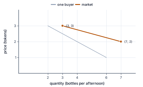
Price in tokens against bottles per afternoon. One buyer plans 6 bottles at 1 token, 4 at 2 and 2 at 3. Adding a second buyer at each common price gives the market points: 7 bottles at 2 tokens and 3 at 3 tokens. Each point pairs one price with one quantity, and a fall in price from 3 to 2 is a move down and to the right along the same schedule.
The figure plots the buyer's schedule and the two market points of this lesson, quantity along the bottom and price up the side.
The conventional market graph puts quantity on the horizontal axis and price on the vertical axis. A table row with price two and quantity seven becomes the point (7,2). Notice that this reverses the common table order of price followed by quantity. Read the axis labels before turning a row into coordinates. The graph represents the same conditional relationship as the table.
When price falls from three to two and quantity rises from three to seven, the point moves down and to the right on a fixed demand curve. This is a movement along the existing relationship. It does not move every point in the schedule. Later, a change in income or preferences may require a new curve; keeping those descriptions separate prevents confusion about the cause of a change.
A plotted point does not show that those purchases have already occurred. Buyers might plan seven bottles while sellers offer only five. Actual transactions then depend on availability and the way buyers and sellers interact. Demand is one side of the market model. Supply and the exchange process are needed to connect desired quantities to possible completed trades.
Graphs also need scales and units. Seven bottles per afternoon differs from seven hundred bottles per week. A line that looks steep on one screen may look flatter when the axes are rescaled, although the underlying schedule has not changed. Interpret economic quantities through the labels and numbers, not through an impression of the picture alone.
Another way: Separate a model from evidence about buyers
A classroom demand table is supplied information. You can calculate exactly what follows from it without claiming that real buyers have the same schedule. To estimate a real schedule, researchers need evidence about choices and about the other influences changing alongside price. A single observed price and sales quantity cannot reveal an entire conditional relationship.
For example, a festival may show both higher drink prices and higher sales than an ordinary day. More visitors and hotter weather could have increased demand at each price. The observation does not automatically prove that raising the drink price caused the higher sales. Comparing scenarios requires attention to the conditions, not just the direction of two recorded numbers.
Stated preferences in a questionnaire and actual purchases can also differ. A person may misunderstand a hypothetical budget or answer differently when spending real resources. This does not make all surveys useless, but it means the type of evidence matters. The schedule in an exercise is a premise; the schedule used for a real decision is a claim that needs support and may be uncertain.
An effective explanation therefore has three parts: identify the supplied price and conditions, read or combine the relevant quantities, and state the limited conclusion. 'At two tokens, these buyers plan seven bottles per afternoon under the given schedule' is more informative than 'demand is seven.' It names what was measured and leaves room for the separate questions of supply, transactions and changing conditions.
5. Planning a fictional refill stand
A school activity uses a fictional refill stand to study demand. The organizers survey two groups about identical refills for one afternoon. At a price of two tokens, group A's supplied schedule gives twelve refills and group B's gives eight. At three tokens the quantities are eight and five. The exercise holds group size, weather, other prices and token budgets fixed.
At two tokens, market quantity demanded is twenty refills. At three tokens it is thirteen. Moving from the higher price to the lower price increases planned purchases by seven. The price falls by one token per refill, not by two tokens just because there are two groups. Each group is evaluated at the same price before its quantity is added to the other group's quantity.
The organizers have capacity for only sixteen refills. That does not change the demand calculation of twenty at two tokens. It creates a separate question about how many trades can occur and how the limited capacity is allocated. We should not replace the desired quantity with capacity and call the replacement demand. Nor can the survey guarantee that exactly twenty refills will be sold on the day.
If a third group arrives, the fixed-buyer assumption no longer holds. The original comparison remains valid for its original groups, but a new market total needs the third group's schedule at each price. This example shows why an accurate result includes the market boundary and the period. The calculation supports a conditional plan, while actual organizing also requires capacity, uncertainty and allocation decisions.
6. A tempting mistake
Demand is the complete conditional schedule. A quantity at one price is quantity demanded; neither a wish list nor an observed sales total automatically supplies that schedule.
7. Read and combine a row
Specify the period.
One afternoon
Both buyers refer to the same interval.
Find the price.
2 tokens
Read quantities at a common own price.
Read A's quantity.
4 bottles
Use the row paired with the stated price.
Read B's quantity.
3 bottles
Use B's row at that same price.
Add the quantities.
4+3=7 bottles
Market demand aggregates quantities, retaining a price of two.
8. Compare two price scenarios
Hold the conditions fixed.
Same buyers, budgets and product
The comparison isolates the own-price change.
Read the higher-price row.
P=3, A=2, B=1
These quantities belong together.
Combine that row.
2+1=3 bottles
Add quantities across buyers.
Combine the lower-price row.
P=2: 4+3=7 bottles
Recompute at the new common price.
Describe the movement.
7-3=4 more bottles
This is a quantity-demanded change on a fixed schedule.
9. Audit a graph and a sales claim
Read the supplied market row.
P=4, Q=6 per day
These are planned purchases under fixed conditions.
Name the horizontal variable.
Q
The conventional market graph places quantity horizontally.
Name the vertical variable.
P
Price belongs vertically in this graph.
Write the ordered pair.
(6,4)
Quantity comes first in the coordinates.
Compare supplied availability.
Only 5 units available
Desired purchases need not equal completed trades.
Bound the conclusion.
Q demanded=6; trades cannot exceed 5 here
The stock limit constrains transactions without rewriting the demand row.
10. Complete a market row
Read the common condition.
P=5 tokens
Both buyers face this price.
Combine their quantities.
6+2=8 units
Both quantities are per afternoon.
Your turn: work this step out. Its working is at the end of the packet.
Retain the market price.
11. Guided practice
At a price of 3 tokens per unit, A plans 5 units and B plans 4 units per afternoon. These are the only buyers, and both face the same price. Enter market quantity and the unchanged price.
Your result
Units per afternoon
Tokens per unit
12. Guided practice
At a common price of three tokens, two buyers plan eight and five units per day. Fill the market total and the graph's horizontal coordinate.
Add the two quantities.
8+5=q
Both plans use the same price and period.
Use quantity on the horizontal axis.
x=q
The conventional market diagram places quantity horizontally.
Keep the stated price vertically.
y=3
Aggregation does not change the own price.
13. Guided practice
Match each description to what it represents under the supplied model.
Demand schedule
Quantity demanded at one price
Observed transactions
Quantities planned at every listed price
Four units planned when price is two
Three units were actually sold yesterday
14. Practice
At a price of 7 tokens per unit, A plans 0 units and B plans 6 units per afternoon. These are the only buyers, and both face the same price. Enter market quantity and the unchanged price.
Units per afternoon: b0
Tokens per unit: b1
15. Practice
At a price of 3 tokens per unit, A plans 8 units and B plans 7 units per afternoon. These are the only buyers, and both face the same price. Enter market quantity and the unchanged price.
Your result
Units per afternoon
Tokens per unit
16. Somewhere new
At a price of 4 tokens per unit, A plans 11 units and B plans 9 units per afternoon. These are the only buyers, and both face the same price. Enter market quantity and the unchanged price.
Your result
Units per afternoon
Tokens per unit
17. Lesson test
Lesson test: one question per skill, one attempt each, no hints. Your answers are checked when you submit.
18. Test question
At a price of 6 tokens per unit, A plans 7 units and B plans 5 units per afternoon. These are the only buyers, and both face the same price. Enter market quantity and the unchanged price.
Units per afternoon: b0
Tokens per unit: b1
19. What you can do now
Explain how to read and aggregate quantities demanded at a common price. Show a fresh example and check its result.