Supply, costs and production time

Paper packet. Every task here also exists on screen, where it is checked automatically; answers written on paper are not assessed by Nydus. When you are back at a device, enter your answers there.

1. What you will learn

2. Starting point

A schedule pairs a price with a planned quantity for a stated period. Production uses scarce resources, so an additional unit can have an additional cost.

3. Words for this lesson

4. An offer is conditional on price and circumstances

Supply describes what sellers plan to offer at a range of possible prices. As with demand, specify the product, unit, participants and period. A supply schedule for identical notebooks per week differs from a count of every notebook currently in a warehouse. The schedule describes offers under conditions; the warehouse count is a stock at a moment.

Suppose a workshop's table lists prices of two, four and six tokens per notebook and weekly quantities of three, seven and nine. At a price of four tokens, its quantity supplied is seven notebooks per week. The whole three-row relationship is supply. Each row is an alternative price scenario, so adding three, seven and nine does not give output for one week.

Willingness and ability both constrain an offer. A seller might like to sell a thousand notebooks but lack the equipment or materials to deliver them. Another seller might have materials available yet prefer a different use of the workshop at a low notebook price. The supplied schedule summarizes these choices under the assumed technology, costs and opportunities.

A plan is not a completed sale. If a workshop offers seven notebooks but buyers purchase five, quantity supplied at the posted price can differ from transactions. Unsold goods might enter inventory, remain unproduced if production follows orders, or be used in another way. The particular arrangement matters. We do not automatically equate an offer, production and sales unless the model explicitly connects them.

Term	What it means
Supply	Quantities sellers are willing and able to offer at different own prices under stated conditions.
Quantity supplied	The quantity offered at one specified price in the stated period.
Marginal cost	The additional cost of producing one more unit or a specified additional batch.
Capacity	A limit on production or delivery during a stated period.
Inventory	A stock of goods held at a particular time.
Market supply	The sum of sellers' offered quantities at a common price and for a common period.

Another way: Additional output can become more costly

A common upward supply schedule reflects the way additional units may become more costly to produce or obtain. The first few units might use readily available materials and regular working time. More output may require less suitable equipment, overtime or resources with better alternative uses. A higher product price can make these additional units worthwhile under the stated model.

Consider a simple producer with additional unit costs of two, three, five and seven tokens. If each unit sells for six tokens and the producer can choose successive units, the first three each add more revenue than cost. The fourth adds seven in cost but only six in revenue. Under this limited model, producing three units maximizes the contribution from these choices. It would be a mistake to produce the fourth merely because total revenue on all four is positive.

The example uses marginal comparisons, not a claim that every producer has exactly this cost pattern. Costs can depend on scale, organization, technology and time. Some outputs are joint products, some capacity comes in indivisible blocks, and some sellers have market power. These features can require a richer model. Here, the schedule states the quantities directly, so we do not infer an unseen cost curve from a few rows.

Opportunity cost belongs in the economic comparison. A resource owned by the producer may have another valuable use even if no money changes hands today. Treating owned resources as automatically costless would distort the production choice. Likewise, a past payment that cannot be recovered should not be counted again as an avoidable cost of one extra unit.

Another way: Read movement along a fixed supply schedule

When the good's own price changes and other relevant influences stay fixed, read a different row of the same supply schedule. In the notebook example, moving from four to six tokens increases quantity supplied from seven to nine per week. This is a change in quantity supplied along the existing relationship. It is not a shift of the entire schedule.

The fixed conditions may include material prices, wages, equipment, technology and the number of sellers. If paper becomes cheaper at the same time as the notebook price changes, the observed output change combines influences. A new schedule may be needed. Separating own-price movement from changes in other conditions will later help explain shifts in market equilibrium.

Do not substitute the buyer's reaction for the seller's. A lower notebook price might encourage buyers to demand more while making some additional production less attractive to sellers. Demand and supply are distinct conditional plans. The market model compares them at a common price; it does not require them to move in the same direction when that price changes.

There may be a range where quantity supplied is unchanged. A seller operating at a strict daily capacity of ten cannot immediately offer twelve merely because price increases. An upward tendency is a useful starting case, but a schedule can include flat quantity responses or other features. Read the actual assumptions and numbers rather than treating a memorized arrow as a substitute for analysis.

Another way: Aggregate compatible offers

Market supply adds the quantities offered by all specified sellers at the same price. If workshop A offers seven notebooks and workshop B offers five at four tokens, market quantity supplied is twelve per week. The common price stays four. Adding the two prices to obtain eight would misdescribe the transaction each buyer faces.

At another price, repeat the addition using that row from both schedules. Suppose at six tokens A offers nine and B offers eight. Market quantity is seventeen. The market schedule now includes the pairs price four, quantity twelve and price six, quantity seventeen. These are alternative market conditions, not two sales totals to combine into one period.

Check for compatible units. An offer of five boxes containing ten notebooks each is fifty notebooks, not five. Daily and weekly flows need a stated time conversion. Products must also meet the same relevant quality and delivery description. A promise to deliver next month cannot simply be added to immediate availability if the market is defined as notebooks delivered this week.

Avoid counting the same goods twice when there is an intermediary. If a wholesaler sells notebooks to a retailer who then sells them to final buyers, adding both offers as independent final supply can duplicate the units. Define the market level before aggregating. The lesson's exercises specify independent sellers offering to the same buyers, so each offered unit is counted once.

Another way: Time changes what can respond

Production flexibility depends on the time available. A stand with ten prepared meals at the start of a short event may be unable to make more before it ends. Over a week, the organizer might buy ingredients and add a shift. Over a year, another kitchen might open. These are different horizons with different feasible responses to price.

This does not mean that every short-run supply curve is vertical or that every long-run supply curve is flat. It means that a model should identify which inputs and decisions can change during its period. A machine may be fixed while working hours vary. Another activity may have almost no scope to change delivery once the event begins. Specific constraints determine the relevant schedule.

Inventory can permit sales without immediate new production. If a shop begins with twenty notebooks, produces ten and sells eighteen, it ends with twelve, assuming no other changes. The inventory account is beginning stock plus additions minus removals. The sales flow of eighteen is not the same as the production flow of ten or the ending stock of twelve.

Keeping these measures separate helps interpret a seller's offer. A short-term increase in sales might draw down inventory rather than indicate increased productive capacity. Conversely, production may rise while sales stay constant because goods are being stored. A statement about supply needs enough context to explain whether it concerns production, offers for sale, or deliveries from an existing stock.

Another way: Plot and interpret without overclaiming

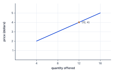
Price in dollars against quantity offered, for a seller who offers 4 units at 2 dollars, 8 at 3, 12 at 4 and 16 at 5. The row price four and quantity twelve becomes the point (12, 4), quantity first. The points rise to the right: under fixed conditions a higher own price brings a larger offered quantity.

The figure plots a supply schedule row by row, with the row at price four and quantity twelve marked as (12, 4).

The conventional supply graph places quantity horizontally and price vertically. A row stating price four and quantity twelve becomes (12,4). The table may list price first, but the coordinate convention requires quantity first. An upward set of points means higher offered quantities at higher own prices under the fixed conditions.

Plot only the points or relationship the model supports. If the case gives three discrete price scenarios, it does not automatically specify every intermediate quantity. A straight line between them can be introduced as an explicit approximation. The visual simplicity of a line is not evidence that sellers have constant responses outside the listed range.

Observed price and sales movements do not reveal supply on their own. A rise in demand can lead both market price and transactions to rise even when the supply schedule itself stays fixed. A technology change can move supply while other conditions move demand. To identify a real supply response, evidence must distinguish these influences rather than read a causal story directly from two observations.

Finish a calculation with units and conditions. 'At four tokens, these two independent workshops offer twelve notebooks per week' states a clear result. It does not assert that twelve will definitely sell, that the price will remain four, or that more production is socially best. The schedule is one part of the market account; the next lesson brings buyers' and sellers' plans together.

5. Offers at a community print workshop

Two fictional print workshops can provide identical booklets for delivery during one week. At a price of three tokens, A offers eight booklets and B offers six. At five tokens, A offers twelve and B offers ten. The model holds paper costs, staffing and equipment fixed and treats the workshops as independent suppliers to the same final market.

Market quantity supplied is fourteen at three tokens and twenty-two at five. The increase is eight booklets per week. Both sellers respond to the same two-token increase in product price; we do not add their prices together. On the conventional graph, the two market points are (14,3) and (22,5).

The event organizer wants eighteen booklets at three tokens. That desire does not turn the fourteen-unit offer into eighteen. It creates a mismatch between the buyer's plan and the sellers' plans under that price. Whether a different price, a later delivery date or another supplier resolves the mismatch is a separate question. The supply arithmetic should remain faithful to the stated conditions.

Now suppose A finds six usable booklets already in storage. If these meet the same quality and delivery requirement and were not included in its offer, it may be able to supply more without printing all of them this week. The case would need a revised offer; the discovery does not justify silently altering the original table. This distinction between stocks, production and offers prevents a common error in interpreting business records. A complete explanation names the time period, common price and source of the supplied quantities.

6. A tempting mistake

Supply is neither all goods that exist nor the number actually sold. It is a conditional offer schedule; a change in the own price moves along it only while its other influences remain fixed.

7. Combine two suppliers

8. Compare additional unit costs

9. Reconcile stock and flows

10. Complete an offer total

11. Guided practice

Independent sellers A and B offer identical units for one week. At the common price of 4 tokens, A offers 7 and B offers 5. Enter total offered quantity and its horizontal coordinate on a graph with quantity horizontal.

12. Guided practice

At one common price, two independent suppliers offer eleven and six units per week. Fill the total and its graph coordinate.

13. Guided practice

Plot the supplied supply schedule as points only, with quantity horizontal and price vertical. Rows (quantity per week, price per unit): (2, 1); (5, 3); (9, 5)

14. Practice

A workshop begins the week with eight finished notebooks, produces six more, offers ten for sale at the stated price, and sells seven. No notebooks are lost or used elsewhere. Enter stock available before sales, new production, quantity offered, actual sales, and ending stock. All quantities count notebooks; production, offers, and sales refer to this week.

15. Practice

Independent sellers A and B offer identical units for one week. At the common price of 5 tokens, A offers 11 and B offers 6. Enter total offered quantity and its horizontal coordinate on a graph with quantity horizontal.

16. Somewhere new

Independent sellers A and B offer identical units for one week. At the common price of 7 tokens, A offers 14 and B offers 9. Enter total offered quantity and its horizontal coordinate on a graph with quantity horizontal.

17. Lesson test

Lesson test: one question per skill, one attempt each, no hints. Your answers are checked when you submit.

18. Test question

At a common price of eight tokens per notebook, workshop A offers thirteen and B offers seven notebooks for the week. A began with nine finished notebooks, produced eleven more, and actually sold ten of its thirteen offered notebooks; no other stock change occurred. Compute total market quantity supplied, A's new production, A's ending inventory, and A's offered-but-unsold quantity. B's production and sales are not supplied and are not needed.

19. What you can do now

Explain how to aggregate supply and distinguish offers, production and inventory. Show a fresh example and check its result.