Consumer surplus, producer surplus and efficiency

Paper packet. Every task here also exists on screen, where it is checked automatically; answers written on paper are not assessed by Nydus. When you are back at a device, enter your answers there.

1. What you will learn

Analyze consumer surplus, producer surplus and efficiency using explicit assumptions, calculated results and a stated limit of the model.

2. Starting point

A competitive equilibrium equates quantity demanded with quantity supplied. Inverse demand gives the price buyers would pay at each quantity; inverse supply gives the price needed to supply it. A triangle's area is one half of its base times its height.

3. Terms and units

4. A transaction can benefit both sides

A buyer willing to pay at most twelve dollars for a unit and a seller willing to accept at least five can both gain by exchanging it for eight dollars. The buyer obtains four dollars of consumer surplus: twelve minus eight. The seller obtains three dollars above the relevant opportunity cost: eight minus five. Together they gain seven dollars, equal to twelve minus five. The price determines how those gains are divided, but for this particular completed trade it does not change their sum.

Willingness to pay is bounded by preferences and purchasing ability. It is not a complete measure of a person's need or social importance. A person with little income may have a low monetary willingness to pay for something extremely important to that person. When the model adds monetary gains across people, it uses a particular efficiency criterion. A distributional judgment may ask additional questions about who receives the benefits and what resources they started with. The arithmetic should not conceal that distinction.

For several discrete buyers, rank willingness-to-pay values from highest to lowest. At a price of eight dollars, buyers whose valuations exceed eight gain positive consumer surplus; a buyer valuing a unit at exactly eight is indifferent in the simple model. The supplied trading convention may specify whether that buyer purchases. Sum each purchasing buyer's valuation minus the actual payment. Do not subtract price from the valuation of people who do not receive the good and then count those amounts as realized surplus.

For several sellers, rank the opportunity costs of supplying units from lowest to highest. At a common price of eight dollars, a unit costing five contributes three to producer surplus and one costing seven contributes one. A unit costing ten will not be voluntarily supplied at eight in the usual competitive model. These discrete comparisons are the building blocks of the continuous surplus areas under demand and above supply. The geometry is a compact way to add many small gains, not a separate economic principle.

Term	What it means
Willingness to pay	The maximum payment a buyer would make for a specified unit under the model.
Consumer surplus	Willingness to pay minus payment, summed over purchased units.
Producer surplus	Receipts minus variable opportunity costs, summed over sold units.
Total surplus	Consumer surplus plus producer surplus in the basic exchange model.
Allocative efficiency	An allocation maximizing the modeled total gains, where marginal social benefit equals marginal social cost.
Deadweight loss	Total gains lost relative to the specified efficient benchmark, rather than a transfer between participants.

Another way: Turn schedules into areas with units

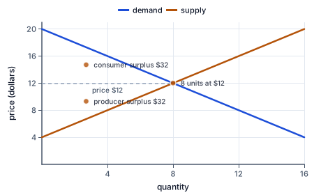
Price in dollars against quantity. Demand P = 20 − Q and supply P = 4 + Q cross at 8 units and 12 dollars. Consumer surplus is the triangle between demand and the 12-dollar price line, base 8 and height 8: 32 dollars. Producer surplus is the triangle between the price line and supply, also base 8 and height 8: 32 dollars. Together they are the 64 dollars of total surplus between the curves.

The figure draws this example: the two 32-dollar triangles sit above and below the 12-dollar price line.

Consider inverse demand P = 20 - Q and inverse supply P = 4 + Q. Their intersection solves 20 - Q = 4 + Q, so quantity is eight and price is twelve dollars. The demand intercept is twenty dollars, and the supply intercept is four. Demand measures marginal willingness to pay; supply represents marginal private opportunity cost under the stipulated competitive conditions. Because this example has no externalities, those private margins also represent the social margins used in the benchmark.

Consumer surplus is the area beneath demand and above the price line, from zero to the eight units purchased. The triangle's base is eight units and its height is twenty minus twelve, or eight dollars per unit. Its area is one half times eight times eight, or thirty-two dollars. Price times quantity is the rectangular payment of ninety-six dollars. That payment is not consumer surplus: buyers surrender it to obtain the goods.

Producer surplus is the area above supply and below the price line over the same output range. Its base is eight, and its height is twelve minus four, also eight. Producer surplus is therefore thirty-two dollars. The cost area below supply includes the opportunity costs of producing the units. Adding the consumer and producer triangles gives total surplus of sixty-four dollars, equal to the full area between demand and supply over the traded range.

The units check is valuable. Quantity multiplied by dollars per unit gives dollars, so an area on this graph measures a total monetary amount. A vertical distance alone is dollars per unit, not total surplus. A common mistake is to report the price gap of eight as the whole gain. Another is to use the full demand intercept of twenty as the consumer triangle's height, which incorrectly includes payments. Identify the actual boundaries of the region before applying an area formula.

Another way: Why the competitive quantity is efficient in this model

At quantities below eight in the example, marginal willingness to pay exceeds marginal cost. An additional unit would create a positive gain equal to that vertical difference. Stopping at six units therefore leaves mutually beneficial transactions unrealized. At quantities above eight, marginal cost exceeds marginal willingness to pay. Producing those extra units uses resources worth more than the benefit the model assigns to them. The intersection separates beneficial increments from harmful ones.

This reasoning establishes allocative efficiency under the supplied assumptions. Buyers and sellers take prices as given, relevant benefits and costs are reflected in the schedules, and the good goes to those whose modeled gains justify receiving it. There are no unpriced spillovers, market power or information problems that change the relationship between private decisions and social margins. Later lessons deliberately relax those assumptions. The competitive result is conditional, not a slogan that every observed market outcome must maximize social well-being.

If output is restricted to six units and the highest-value buyers trade with the lowest-cost sellers, the missing units from six to eight create deadweight loss. At quantity six, demand is fourteen dollars and supply is ten, so their vertical gap is four. At quantity eight the gap is zero. The lost-gains triangle therefore has base two units and height four dollars per unit. Its area is one half times two times four, or four dollars. Writing both schedule values prevents a remembered intercept difference from replacing the relevant local gap.

Allocation among participants also matters. If a low-value buyer receives a scarce unit while a higher-value buyer is excluded, total surplus can be lower even when the total quantity is unchanged. A quantity calculation alone cannot determine the exact loss under arbitrary rationing. A model that computes surplus from the usual demand area implicitly allocates units to the highest willingness-to-pay uses. If a price-control problem specifies random rationing or costly lines, the analysis must include those rules rather than silently using the efficient allocation benchmark.

Another way: Transfers, profit and distribution are different records

A change in price can transfer surplus between buyers and sellers on units still traded. Suppose the same eight units are exchanged at thirteen rather than twelve dollars, with the same buyers and sellers. Buyers pay eight dollars more in total and sellers receive eight dollars more. Consumer surplus falls by eight and producer surplus rises by eight; total surplus on those fixed transactions is unchanged. Whether such a price is sustainable under the market's rules is a separate question. This thought experiment isolates the distributional effect of a transfer.

Deadweight loss instead concerns gains that disappear rather than merely change recipients. A policy that reduces beneficial trades can create such a loss even while generating government revenue. In a later tax model, tax receipts will be added to private surplus when calculating the benchmark total. Counting all tax revenue as lost wealth would confuse a payment to another participant with a destroyed gain. Administrative resources and behavioral distortions may create costs, but they must be modeled separately.

Producer surplus should not automatically be called economic profit. In the standard short-run firm interpretation, producer surplus is revenue minus variable cost. Economic profit also subtracts fixed opportunity costs. A business receiving thirty-two dollars of producer surplus and facing twenty dollars of fixed economic cost has twelve dollars of economic profit. If fixed cost were forty, profit would be negative eight even though producer surplus remained positive. The distinction becomes essential when deciding whether a firm should operate temporarily or exit in the long run.

Efficiency and equity can conflict, coincide or simply concern different dimensions. Two policies may generate the same modeled total surplus while dividing it differently. A policy with lower total surplus might be preferred under an explicit distributional objective. Economics can identify the trade-off without declaring that the efficiency criterion is the only legitimate objective. Report whose surplus changes, by how much, what costs are included and which criterion supports the conclusion.

Finally, avoid treating willingness-to-pay estimates as perfectly known facts merely because an exercise supplies exact numbers. In real applications, demand schedules are estimated and may omit nonmarket benefits or depend on income distributions. An analyst should test sensitivity to plausible alternatives. The exact triangle calculation is a useful skill, but its precision is conditional on the model inputs and assumptions that define the region being measured.

5. Auditing a fictional equipment exchange

A community equipment exchange models demand for refurbished lamps as P = 20 - Q and supply as P = 4 + Q, with prices in dollars and quantities per event. The competitive benchmark is eight lamps at twelve dollars. Consumer surplus is thirty-two dollars, producer surplus is thirty-two dollars, and total modeled gains are sixty-four dollars. The exchange coordinator records these as different entries instead of treating the ninety-six dollars of sales revenue as the benefit created.

Suppose a storage restriction permits only six lamps to be exchanged. If the six highest-value uses receive the six lowest-cost lamps, the two omitted units would have created four dollars of additional gains. The total surplus falls from sixty-four to sixty dollars. This is the efficient-rationing benchmark for the restriction, not a guarantee about every possible allocation of six lamps. If a low-value use displaces a high-value use, additional gains can be lost.

The coordinator then asks whether a donation that transfers eight dollars from buyers to refurbishers would alter the production opportunity costs or the recipients of lamps. If it merely changes payments on the same trades, it redistributes surplus without changing the sixty-dollar total for that restricted allocation. If the payment induces another lamp to be repaired, the quantity effect must be calculated separately. The same financial transfer can therefore have both an accounting role and an incentive effect, depending on the rules.

The report should not describe the highest-surplus arrangement as automatically the fairest. Participants may care about access for households with limited income or about compensating volunteers. Those objectives can be stated alongside the surplus calculation. Keeping the accounts separate makes disagreement more precise: people can agree on the model's gains and still choose different distributional priorities.

6. Check the tempting shortcut

Sales revenue is not total surplus. A payment that changes recipients is not automatically deadweight loss. Producer surplus excludes fixed cost, while economic profit deducts it. The efficiency benchmark also depends on how scarce units are allocated, not only how many are produced.

7. In the fictional Alder model, inverse demand is P=22-Q and inverse supply is P=6+Q, in dollars per unit. Competition clears this market; no externalities, market power or rationing are present. Calculate equilibrium price, consumer surplus, and producer surplus in dollars. Treat quantities as divisible and the curves as continuous.

8. In the fictional Birch model, inverse demand is P=24-Q and inverse supply is P=8+Q, in dollars per unit. Competition clears this market; no externalities, market power or rationing are present. Calculate equilibrium price, consumer surplus, and producer surplus in dollars. Treat quantities as divisible and the curves as continuous.

9. In the fictional Cedar model, inverse demand is P=26-Q and inverse supply is P=10+Q, in dollars per unit. Competition clears this market; no externalities, market power or rationing are present. Calculate equilibrium price, consumer surplus, and producer surplus in dollars. Treat quantities as divisible and the curves as continuous.

10. In the fictional Dune model, inverse demand is P=28-Q and inverse supply is P=12+Q, in dollars per unit. Competition clears this market; no externalities, market power or rationing are present. Calculate equilibrium price, consumer surplus, and producer surplus in dollars. Treat quantities as divisible and the curves as continuous.

11. Guided practice

In the fictional Elm model, inverse demand is P=30-Q and inverse supply is P=14+Q, in dollars per unit. Competition clears this market; no externalities, market power or rationing are present. Calculate equilibrium price, consumer surplus, and producer surplus in dollars. Treat quantities as divisible and the curves as continuous.

12. Guided practice

In the fictional Dune model, inverse demand is P=28-Q and inverse supply is P=12+Q, in dollars per unit. Competition clears this market; no externalities, market power or rationing are present. Calculate equilibrium price, consumer surplus, and producer surplus in dollars. Treat quantities as divisible and the curves as continuous.

13. Guided practice

In the fictional Fern model, inverse demand is P=32-Q and inverse supply is P=16+Q, in dollars per unit. Competition clears this market; no externalities, market power or rationing are present. Calculate equilibrium price, consumer surplus, and producer surplus in dollars. Treat quantities as divisible and the curves as continuous.

14. Practice

In the fictional Grove model, inverse demand is P=34-Q and inverse supply is P=18+Q, in dollars per unit. Competition clears this market; no externalities, market power or rationing are present. Calculate equilibrium price, consumer surplus, and producer surplus in dollars. Treat quantities as divisible and the curves as continuous.

15. Practice

In the fictional Harbor model, inverse demand is P=36-Q and inverse supply is P=20+Q, in dollars per unit. Competition clears this market; no externalities, market power or rationing are present. Calculate equilibrium price, consumer surplus, and producer surplus in dollars. Treat quantities as divisible and the curves as continuous.

16. Somewhere new

A community equipment exchange wants to distinguish its sales receipts from the gains created for buyers and refurbishers. Treat its schedules as marginal willingness to pay and marginal opportunity cost, and calculate the two surplus accounts without treating their sum as a fairness judgment. In the fictional Island model, inverse demand is P=38-Q and inverse supply is P=22+Q, in dollars per unit. Competition clears this market; no externalities, market power or rationing are present. Calculate equilibrium price, consumer surplus, and producer surplus in dollars. Treat quantities as divisible and the curves as continuous.

17. Lesson test

Lesson test: one question per skill, one attempt each, no hints. Your answers are checked when you submit.

18. Test question

In the fictional Juniper model, inverse demand is P=40-Q and inverse supply is P=24+Q, in dollars per unit. Competition clears this market; no externalities, market power or rationing are present. Calculate equilibrium price, consumer surplus, and producer surplus in dollars. Treat quantities as divisible and the curves as continuous.

19. What you can do now

Reconstruct the model without the worked example. Explain each requested measure's units and identify an assumption that the conclusion depends on.

Working for the steps left to you