Demand, supply and equilibrium changes

Paper packet. Every task here also exists on screen, where it is checked automatically; answers written on paper are not assessed by Nydus. When you are back at a device, enter your answers there.

1. What you will learn

Analyze demand, supply and equilibrium changes using explicit assumptions, calculated results and a stated limit of the model.

2. Starting point

A budget limits what consumers can purchase, while production costs constrain sellers. A linear equation describes a whole schedule. To find an intersection, solve the two equations simultaneously rather than reading only one side of the market.

3. Terms and units

4. Two plans meet in a market

Demand is a schedule of intended purchases at alternative prices. It is not one transaction, one person's desire or the amount already sold. A consumer might want a product intensely but lack the budget to buy it. The demand schedule records quantities the buyers would purchase under the stated conditions. In the standard downward-sloping case, a lower own price increases quantity demanded, other determinants unchanged. The schedule concerns a specified good, market and time period: cups per day cannot be compared directly with cups per month without converting units.

Supply is the corresponding schedule of intended sales. Sellers may be willing to provide more output at a higher price because the additional units cover higher opportunity costs. That familiar upward relationship depends on the market and relevant time horizon; it is not a claim that every conceivable supply curve must have the same shape. Our first model uses an upward-sloping linear supply schedule and a downward-sloping linear demand schedule so their intersection is transparent.

Market demand can be assembled by adding buyers' quantities at the same price. If one buyer would purchase three units at eight dollars and another would purchase two, their combined quantity demanded at eight dollars is five. This is horizontal addition because quantity lies on the horizontal axis. Do not add the two prices or average the quantities. Market supply can likewise add different sellers' offered quantities at each common price. Later, a public-good lesson will explain why its benefit curves require a different aggregation procedure.

A graph convention places price vertically and quantity horizontally. An equation such as Qd = 40 - 2P solves quantity in terms of price. To graph inverse demand, rearrange it as P = 20 - Q/2. Both describe the same relationship over the relevant nonnegative range. A model should not be extended mechanically into negative quantities where its intended economic interpretation no longer applies. Check both the axes and the domain before treating an algebraic result as a feasible market outcome.

Term	What it means
Demand	The relationship between price and quantities buyers would purchase, other relevant determinants held fixed.
Supply	The relationship between price and quantities sellers would offer, other relevant determinants held fixed.
Equilibrium	A price and quantity at which planned purchases equal planned sales.
Shortage	Quantity demanded minus quantity supplied when that difference is positive.
Surplus of goods	Quantity supplied minus quantity demanded when that difference is positive.
Comparative statics	A comparison of equilibria before and after a specified change, without a full account of the adjustment path.

Another way: Equilibrium is a compatibility condition

Suppose quantity demanded is Qd = 40 - 2P and quantity supplied is Qs = 2P. At equilibrium, the same quantity must satisfy both plans at the same price. Setting 40 - 2P = 2P gives 40 = 4P, so P = 10 dollars. Substituting that price into either equation gives Q = 20 units. Substitution into both equations is a useful check: each must produce twenty. A price without a corresponding quantity is only part of the equilibrium answer.

At a price of eight dollars, quantity demanded is twenty-four while quantity supplied is sixteen. The shortage is eight units. The word shortage describes excess demand at that price; it is not a statement that the product has disappeared from the economy altogether. In a competitive adjustment story without binding restrictions, some buyers offer more or sellers recognize they can raise price. A higher price reduces quantity demanded and increases quantity supplied, tending to narrow the gap.

At twelve dollars, quantity demanded is sixteen while quantity supplied is twenty-four. The excess supply is eight units. Sellers may lower their offers to attract purchasers or cut production. Again, the schedules describe intended purchases and sales, not a guarantee that twenty-four units are actually exchanged. When buyers want only sixteen at the prevailing price, identifying the actual trades may require a trading or rationing mechanism. The equilibrium exercise avoids that complication by finding the price at which plans agree.

Equilibrium does not mean that every buyer is happy, that everyone obtains a desired product, or that the allocation is fair. Some people may value a unit but be unable or unwilling to pay the market price. Equilibrium is also not a claim that the economy never changes. It is a condition within a model with specified determinants. When one of those determinants changes, the old equality may no longer hold. The model then predicts a different intersection, subject to its assumptions about competition, adjustment and institutions.

Another way: Movement along a curve or movement of a curve

An own-price change moves along a fixed demand curve. If a product's price falls from ten to eight dollars and purchases rise along Qd = 40 - 2P, that is an increase in quantity demanded. Calling it an increase in demand obscures the distinction between a new point on the same relationship and a different relationship. An increase in demand means buyers want more at each price, represented by a rightward shift of the demand curve.

Several determinants can shift demand. Higher income raises demand for a normal good but lowers demand for an inferior good. A higher price of a substitute can increase demand for this good, while a higher price of a complement can decrease it. Changes in tastes, expectations or the number of buyers can also shift the schedule. These directions depend on how the goods are related and on the particular assumption. For example, expecting a future price increase may raise present purchases of a storable item, but storage limitations can matter.

Supply shifts when a determinant other than the good's own price changes. A lower input price or a productivity improvement can make it worthwhile to offer more at every output price. An increase in a relevant input cost can reduce supply. Taxes, subsidies, expectations and the number of sellers may also affect the schedule. State the causal link rather than memorizing an isolated arrow: lower unit costs allow more units to be produced profitably at a given selling price.

Suppose demand changes from Qd = 40 - 2P to Qd = 48 - 2P while supply remains Qs = 2P. The new equilibrium solves 48 - 2P = 2P, giving P = 12 and Q = 24. Demand has shifted outward; the resulting price increase produces a movement along the unchanged supply curve. There is no need to invent a second supply shift to explain the higher quantity supplied. Keeping the original cause separate from the price-mediated response is central to comparative statics.

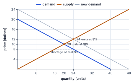
Price in dollars against quantity in units. Demand Qd = 40 - 2P falls and supply Qs = 2P rises; they cross at 20 units and 10 dollars. At 8 dollars buyers want 24 and sellers offer 16, a shortage of 8. Demand shifted out to Qd = 48 - 2P crosses the same supply curve at 24 units and 12 dollars.

Read the chart with price up the side. The two solid curves cross at 20 units and 10 dollars, the same answer the algebra gave. The dashed guide at 8 dollars runs from supply at 16 units to demand at 24: its length is the shortage. The faint curve is the new demand; follow the supply curve up from the old crossing to the new one at 24 units and 12 dollars, which is the movement along supply the shift causes.

Another way: What a pair of shifts can and cannot establish

With the usual slopes, an increase in demand alone raises both equilibrium price and quantity. An increase in supply alone lowers equilibrium price and raises quantity. A decrease in demand lowers both price and quantity; a decrease in supply raises price and lowers quantity. These directional results follow from the supplied curve shapes and the condition that the other curve remains unchanged. They are not unconditional forecasts about a real market in which several determinants may change together.

When demand and supply both increase, their quantity effects reinforce one another, so equilibrium quantity rises under the standard model. Their price effects oppose one another. Without information about the size and shape of the shifts, the price change is indeterminate: it can rise, fall or remain unchanged. 'Indeterminate' does not mean no answer is possible in principle. It means the given directional information is insufficient. Numerical schedules can resolve the uncertainty by specifying the relative shifts.

Suppose original demand is 40 - 2P and original supply is 2P. New demand is 48 - 2P and new supply is 8 + 2P. Equating the new schedules gives 48 - 2P = 8 + 2P, hence P = 10 and Q = 28. Both curves shift right, quantity rises and price stays unchanged in this particular calculation. If supply shifted by only four units instead of eight, price would rise. The direction-only case and the numerical case therefore ask different questions.

An observed price-and-quantity pair does not uniquely identify its cause. A higher price with a higher quantity is consistent with an outward demand shift and unchanged supply, but a combination of other shifts may produce the same observation. Identification requires additional evidence or restrictions. A useful classroom habit is to distinguish 'the model predicts this outcome under the stated shock' from 'this observation proves that shock occurred.' The second claim reverses the inference and generally needs more support.

Comparative statics also leaves the path between equilibria undescribed. It does not specify whether prices adjust within minutes or months, whether inventories buffer the change, or whether some firms exit along the way. Those details require a dynamic or institutional model. For the present task, report the initial schedules, the specified change, the new intersection and the assumptions holding the rest constant. This produces a complete answer to the model's question without pretending to answer every question about the market.

5. A repair market after a new delivery service

A fictional neighborhood has a market for bicycle repairs measured per week. Before a delivery cooperative opens, demand is Qd = 40 - 2P and supply is Qs = 2P, with price measured in dollars per repair. The equilibrium is ten dollars and twenty repairs. The cooperative's bicycles create additional demand at every price, represented by Qd = 48 - 2P. Repair methods, input prices and the number of repairers remain unchanged. The new equilibrium is twelve dollars and twenty-four repairs.

The explanation has two stages. The cooperative changes the demand schedule; that is the initiating shift. The resulting higher price makes repairers willing to supply more along their existing supply curve. Saying that 'supply increased because more repairs were sold' would confuse that movement with a shift. To claim a supply shift, the report would need a separate cause such as new repair equipment, a lower parts cost or additional repair businesses.

Now add an explicit productivity improvement that changes supply to Qs = 8 + 2P. With the new demand, the equilibrium returns to ten dollars while quantity rises to twenty-eight. The same demand increase therefore accompanies different price outcomes depending on what happens to supply. A report that records only the final price of ten dollars might miss substantial changes in the market's underlying conditions.

These invented equations make the comparison exact. They do not predict a real neighborhood's response to a delivery service. A real study would need data on repairs, prices, input costs and other changes, and would need to consider whether repairers can adjust capacity over the relevant period. The model nevertheless improves the investigation by separating possible mechanisms and showing which additional evidence could distinguish them.

6. Check the tempting shortcut

Quantity demanded is a point on demand; demand is the relationship itself. A price-mediated movement along unchanged supply is not a supply shift. When simultaneous shifts push price in opposite directions, report the ambiguity unless their magnitudes are supplied.

7. In the fictional Alder model, quantity demanded is Qd=44-2P and quantity supplied is Qs=2P, with price P in dollars and quantity in units per day. Then demand becomes Qd=52-2P while supply is unchanged. Both schedules apply over the relevant positive quantities. Calculate the initial equilibrium price, new equilibrium price, and new equilibrium quantity.

8. In the fictional Birch model, quantity demanded is Qd=48-2P and quantity supplied is Qs=2P, with price P in dollars and quantity in units per day. Then demand becomes Qd=56-2P while supply is unchanged. Both schedules apply over the relevant positive quantities. Calculate the initial equilibrium price, new equilibrium price, and new equilibrium quantity.

9. In the fictional Cedar model, quantity demanded is Qd=52-2P and quantity supplied is Qs=2P, with price P in dollars and quantity in units per day. Then demand becomes Qd=60-2P while supply is unchanged. Both schedules apply over the relevant positive quantities. Calculate the initial equilibrium price, new equilibrium price, and new equilibrium quantity.

10. In the fictional Dune model, quantity demanded is Qd=56-2P and quantity supplied is Qs=2P, with price P in dollars and quantity in units per day. Then demand becomes Qd=64-2P while supply is unchanged. Both schedules apply over the relevant positive quantities. Calculate the initial equilibrium price, new equilibrium price, and new equilibrium quantity.

11. Guided practice

In the fictional Elm model, quantity demanded is Qd=60-2P and quantity supplied is Qs=2P, with price P in dollars and quantity in units per day. Then demand becomes Qd=68-2P while supply is unchanged. Both schedules apply over the relevant positive quantities. Calculate the initial equilibrium price, new equilibrium price, and new equilibrium quantity.

12. Guided practice

In the fictional Dune model, quantity demanded is Qd=56-2P and quantity supplied is Qs=2P, with price P in dollars and quantity in units per day. Then demand becomes Qd=64-2P while supply is unchanged. Both schedules apply over the relevant positive quantities. Calculate the initial equilibrium price, new equilibrium price, and new equilibrium quantity.

13. Guided practice

In the fictional Fern model, quantity demanded is Qd=64-2P and quantity supplied is Qs=2P, with price P in dollars and quantity in units per day. Then demand becomes Qd=72-2P while supply is unchanged. Both schedules apply over the relevant positive quantities. Calculate the initial equilibrium price, new equilibrium price, and new equilibrium quantity.

14. Practice

In the fictional Grove model, quantity demanded is Qd=68-2P and quantity supplied is Qs=2P, with price P in dollars and quantity in units per day. Then demand becomes Qd=76-2P while supply is unchanged. Both schedules apply over the relevant positive quantities. Calculate the initial equilibrium price, new equilibrium price, and new equilibrium quantity.

15. Practice

In a fictional market, inverse demand is P=24-Q, with P in dollars per unit and Q in units per day. Plot demand at Q=0, Q=8 and Q=16. Quantity belongs on the horizontal axis. Other demand determinants are fixed.

16. Somewhere new

A new delivery cooperative increases demand for bicycle repairs. Repair equipment, parts prices and the number of repairers remain unchanged. Use the before-and-after schedules to distinguish the initiating demand shift from repairers' movement along unchanged supply. In the fictional Island model, quantity demanded is Qd=76-2P and quantity supplied is Qs=2P, with price P in dollars and quantity in units per day. Then demand becomes Qd=84-2P while supply is unchanged. Both schedules apply over the relevant positive quantities. Calculate the initial equilibrium price, new equilibrium price, and new equilibrium quantity.

17. Lesson test

Lesson test: one question per skill, one attempt each, no hints. Your answers are checked when you submit.

18. Test question

In the fictional Juniper model, quantity demanded is Qd=80-2P and quantity supplied is Qs=2P, with price P in dollars and quantity in units per day. Then demand becomes Qd=88-2P while supply is unchanged. Both schedules apply over the relevant positive quantities. Calculate the initial equilibrium price, new equilibrium price, and new equilibrium quantity.

19. What you can do now

Reconstruct the model without the worked example. Explain each requested measure's units and identify an assumption that the conclusion depends on.

Working for the steps left to you

	Calculated value
Initial price
New price
New quantity

	Calculated value
Initial price
New price
New quantity

	Calculated value
Initial price
New price
New quantity