Derived demand and competitive factor markets

Paper packet. Every task here also exists on screen, where it is checked automatically; answers written on paper are not assessed by Nydus. When you are back at a device, enter your answers there.

1. What you will learn

Analyze derived demand and competitive factor markets using explicit assumptions, calculated results and a stated limit of the model.

2. Starting point

Marginal product measures extra physical output from an additional input. A competitive product seller receives the same price on each extra unit. Profit-maximizing decisions compare additional revenue with additional opportunity cost.

3. Terms and units

4. Input demand begins with the product

A firm typically hires labor or rents equipment because the input helps produce something that generates revenue or serves the organization's stated objective. In a profit-maximization model, demand for the input is derived from the demand for that output and the input's productive contribution. A worker's physical productivity alone does not determine the employer's willingness to pay. The revenue obtained from the additional output also matters.

Suppose an additional worker produces six extra units of a product. If each extra unit brings three dollars of revenue, the worker adds eighteen dollars to revenue. If the product price falls to two dollars while physical productivity remains six, the additional revenue falls to twelve. The technology did not deteriorate, yet the employer's derived demand for labor is lower. This example separates a physical contribution from its market valuation.

Marginal revenue product, or MRP, is marginal product multiplied by marginal revenue from the output. When the firm is a price taker in the product market, marginal revenue equals product price, so MRP = MP times P. When the firm has product-market power, marginal revenue generally differs from price, and the correct revenue-product expression uses MR. Applying MP times the posted price to a single-price monopolist can overstate the revenue from extra output because expanding sales affects earlier receipts.

Factor markets include more than labor. A firm can compare the additional revenue from another machine-hour with its rental cost, or the output contribution of land with its opportunity cost. The principles are similar, though the measurement, adjustment time and institutional rules differ. This lesson uses labor to make the sequence concrete while keeping the broader derived-demand logic visible.

Term	What it means
Factor of production	An input such as labor, land or productive capital used to produce output.
Derived demand	Demand for an input arising from the value and demand for the output it helps produce.
Marginal revenue product	The additional revenue generated by an additional unit of an input.
Marginal factor cost	The increase in total input expenditure caused by using an additional input unit.
Competitive labor market	A model in which an individual employer and worker take the relevant wage as given.
Human capital	Skills and knowledge embodied in people that can affect productive capabilities.
Economic rent	A payment above the opportunity cost required to keep a resource in its current use.

Another way: Solve the firm's hiring increments

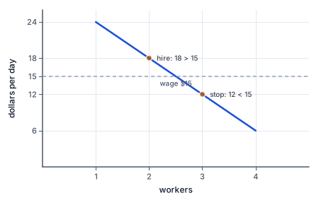
Dollars per day against workers hired. At 3 dollars a unit, four successive workers add products worth 24, 18, 12 and 6 dollars. The competitive wage is 15 dollars. The first two workers bring in more than they cost; the third brings in 12, less than 15, so the firm hires two.

The figure plots the four workers' marginal revenue products against the fifteen-dollar wage: hire while the point lies above the line.

Consider a competitive product seller receiving three dollars per unit. Successive workers add eight, six, four and two units per day with the same fixed equipment. Their marginal revenue products are twenty-four, eighteen, twelve and six dollars. If the competitive daily wage is fifteen dollars for every worker, the first and second workers add more revenue than cost. The third adds only twelve dollars while costing fifteen, so the firm stops after two under the stated discrete model.

Total wage expenditure is two times fifteen, or thirty dollars. It is not the second worker's MRP and not the sum of the two MRP values. The sum of the accepted marginal revenue products is forty-two dollars, the total additional revenue attributed to those two workers relative to zero labor in the supplied sequence. Subtracting the wage bill gives a twelve-dollar contribution before any other costs designated fixed in the comparison.

For divisible inputs in a smooth interior solution on the relevant declining-MRP range, the hiring condition is MRP = marginal factor cost. In a competitive labor market, the individual employer faces a constant wage, so marginal factor cost equals that wage. With discrete workers, equality may not occur. Accept increments whose MRP exceeds cost and reject the next increment that reduces profit, checking feasible boundaries and any specified tie convention.

The condition describes the firm's choice under supplied objectives and market rules. It does not measure a person's moral worth or every contribution that work makes to society. Unpaid care, external benefits and institutional constraints may not appear in the firm's revenue. Even within market production, teamwork and measurement difficulties can complicate attributing output to an individual. The classroom table stipulates increments to isolate the decision logic, rather than claiming all real workers' contributions are directly observable.

Another way: Firm and market labor curves are different

An individual competitive employer takes the market wage as given and can hire the relevant quantity at that wage. Its labor-supply curve is horizontal over the modeled range. The labor market as a whole can have an upward-sloping supply curve because higher wages attract more hours or participants from other uses. Just as a competitive firm's product demand differs from market demand, its input-supply condition differs from aggregate labor supply.

Market labor demand aggregates employers' demands at each wage, with care about changes in product prices and other conditions when the whole industry expands. In a simple classroom market, we take the supplied market schedule as given. Its intersection with labor supply determines the equilibrium wage and employment. The firm's hiring calculation then uses that wage. Mixing a market wage equation with one firm's marginal-product table without specifying how they relate can answer an ill-defined question.

The market supply of labor can shift with changes in the number of qualified workers, migration within the modeled setting, alternative wages, preferences over work and leisure, or training opportunities. A higher wage in another occupation can make this occupation less attractive at each own wage, shifting its supply inward. A change in this occupation's own wage is instead a movement along its existing supply schedule, other determinants held fixed.

Individual labor supply can involve both substitution and income effects. A higher wage raises the opportunity cost of leisure, encouraging work through substitution. It also increases purchasing power for a given amount of work, which can encourage more leisure if leisure is a normal good. The net effect is not universally positive for every individual and wage range. The basic upward-sloping market supply used in an activity is an explicit model assumption, not a theorem that every person always works more at a higher wage.

Another way: Track shifts in derived demand

An increase in demand for a firm's product can raise its price or marginal revenue, increasing the revenue value of labor's physical product. A productivity improvement can increase marginal product and shift labor demand outward, other things equal. A fall in output demand can work in the opposite direction. These are shifts of the MRP relationship, distinct from moving along an unchanged relationship when the wage changes.

Other input prices can have competing effects. If a machine becomes cheaper and substitutes for labor in a given production task, the firm may use fewer workers for that task. But lower production cost can also expand output and increase demand for some labor. Whether the overall labor-demand effect is positive or negative depends on the technology, substitution possibilities and scale response. A simple statement that 'cheaper capital always reduces labor demand' would omit the second mechanism.

Complementary inputs can raise one another's productivity. Better equipment may make a worker more productive rather than replace the worker. Training can also change productive capability, though its cost and who finances it matter. A complete investment comparison considers future benefits and opportunity costs, not just a current wage difference. In this lesson we do not make personal career or financial recommendations; we identify how supplied changes affect an input-demand model.

Differences in observed wages can reflect productivity, working conditions, required training, scarcity, institutions, bargaining power or discrimination, among other factors. A competitive marginal-product benchmark does not prove that every observed wage difference is justified or caused by productivity alone. Establishing a cause requires evidence and an appropriate comparison. The model supplies a conditional relationship, not a universal explanation of inequality.

Economic rent distinguishes a resource's payment from the minimum needed to retain it in the current use. If a worker would remain in an occupation at a lower wage than the actual payment, the difference can be described as rent in that model. Opportunity costs vary across people and alternatives, so this is not a moral label or a claim that the payment was unearned. The concept helps analyze how a change in scarcity or policy affects resource owners.

An effective factor-market answer follows a chain: specify the product-market revenue condition, calculate physical marginal products, convert them into MRP, identify the input's marginal cost, and compare feasible hiring increments. A market-level answer additionally solves the wage from labor demand and supply. Keeping each link explicit makes it possible to see whether a changed conclusion came from technology, output demand, input-market conditions or a different institutional assumption.

Another way: Use the same time basis throughout

An hourly wage cannot be compared directly with a daily marginal revenue product. Convert both into the same period or define a worker-hour as the input unit. Likewise, a worker hired for several hours may have different marginal productivity across those hours. The finite table treats each listed worker-day as one indivisible increment. Its answer should retain that unit rather than silently reinterpret the number as a headcount for an unspecified period.

5. A fictional workshop hires for a fixed production line

A fictional workshop sells its output competitively at three dollars per unit. One fixed line with successive workers adds eight, six, four and two units per day. The workers' MRP values are therefore twenty-four, eighteen, twelve and six dollars. At a common daily wage of fifteen, two workers maximize the supplied finite contribution: the first two increments exceed the wage, while the third does not. The wage bill is thirty dollars, and the added revenue from those workers is forty-two.

Suppose product demand weakens and the competitive price falls to two dollars, with the physical production table unchanged. MRP values become sixteen, twelve, eight and four. At the same fifteen-dollar wage, only the first worker's increment remains worthwhile. The reduced hiring is caused by lower revenue per unit of output, not by a change in the workers' physical productivity. That distinction is what derived demand is designed to express.

Alternatively, suppose a new tool raises the third worker's marginal product from four to six while the original three-dollar price and fifteen-dollar wage remain. The third MRP becomes eighteen and hiring that worker now adds three dollars to the contribution. This comparison changes technology while holding the revenue and wage conditions fixed.

The exercise does not establish the appropriate wage for real workers or evaluate their social worth. It isolates a private employer's choice with exact hypothetical increments and no additional variable inputs. A real study would need to examine measurement, teamwork, working conditions, institutions and possible external effects. The model's value is that it separates the physical, revenue and cost components of a hiring decision so each can be questioned or revised explicitly.

6. Check the tempting shortcut

Marginal product is physical output; marginal revenue product is revenue. MP times price requires a price-taking product seller. The firm's horizontal labor supply is not the whole market's supply, and a conditional productivity model does not explain every observed wage difference.

7. In the fictional Alder model, a competitive seller receives 3 dollars per unit. Successive workers add outputs [8, 6, 4, 2] units per day. A competitive labor market lets the firm hire any number at wage 15 dollars each per day. Workers are indivisible and the fixed input is unchanged. Calculate the second worker's marginal revenue product, the profit-maximizing number hired, and its total wage bill. Ignore all other variable inputs.

8. In the fictional Birch model, a competitive seller receives 4 dollars per unit. Successive workers add outputs [8, 6, 4, 2] units per day. A competitive labor market lets the firm hire any number at wage 20 dollars each per day. Workers are indivisible and the fixed input is unchanged. Calculate the second worker's marginal revenue product, the profit-maximizing number hired, and its total wage bill. Ignore all other variable inputs.

9. In the fictional Cedar model, a competitive seller receives 5 dollars per unit. Successive workers add outputs [8, 6, 4, 2] units per day. A competitive labor market lets the firm hire any number at wage 25 dollars each per day. Workers are indivisible and the fixed input is unchanged. Calculate the second worker's marginal revenue product, the profit-maximizing number hired, and its total wage bill. Ignore all other variable inputs.

10. In the fictional Dune model, a competitive seller receives 6 dollars per unit. Successive workers add outputs [8, 6, 4, 2] units per day. A competitive labor market lets the firm hire any number at wage 30 dollars each per day. Workers are indivisible and the fixed input is unchanged. Calculate the second worker's marginal revenue product, the profit-maximizing number hired, and its total wage bill. Ignore all other variable inputs.

11. Guided practice

In the fictional Elm model, a competitive seller receives 7 dollars per unit. Successive workers add outputs [8, 6, 4, 2] units per day. A competitive labor market lets the firm hire any number at wage 35 dollars each per day. Workers are indivisible and the fixed input is unchanged. Calculate the second worker's marginal revenue product, the profit-maximizing number hired, and its total wage bill. Ignore all other variable inputs.

12. Guided practice

In the fictional Dune model, a competitive seller receives 6 dollars per unit. Successive workers add outputs [8, 6, 4, 2] units per day. A competitive labor market lets the firm hire any number at wage 30 dollars each per day. Workers are indivisible and the fixed input is unchanged. Calculate the second worker's marginal revenue product, the profit-maximizing number hired, and its total wage bill. Ignore all other variable inputs.

13. Guided practice

In the fictional Fern model, a competitive seller receives 8 dollars per unit. Successive workers add outputs [8, 6, 4, 2] units per day. A competitive labor market lets the firm hire any number at wage 40 dollars each per day. Workers are indivisible and the fixed input is unchanged. Calculate the second worker's marginal revenue product, the profit-maximizing number hired, and its total wage bill. Ignore all other variable inputs.

14. Practice

In the fictional Grove model, a competitive seller receives 9 dollars per unit. Successive workers add outputs [8, 6, 4, 2] units per day. A competitive labor market lets the firm hire any number at wage 45 dollars each per day. Workers are indivisible and the fixed input is unchanged. Calculate the second worker's marginal revenue product, the profit-maximizing number hired, and its total wage bill. Ignore all other variable inputs.

15. Practice

In the fictional Harbor model, a competitive seller receives 10 dollars per unit. Successive workers add outputs [8, 6, 4, 2] units per day. A competitive labor market lets the firm hire any number at wage 50 dollars each per day. Workers are indivisible and the fixed input is unchanged. Calculate the second worker's marginal revenue product, the profit-maximizing number hired, and its total wage bill. Ignore all other variable inputs.

16. Somewhere new

A repair enterprise sells output competitively and can recruit staff at a fixed daily wage. A manager has mistakenly called physical packages per worker a dollar contribution. Convert the productivity increments into revenue before calculating the hiring choice and wage bill. In the fictional Island model, a competitive seller receives 11 dollars per unit. Successive workers add outputs [8, 6, 4, 2] units per day. A competitive labor market lets the firm hire any number at wage 55 dollars each per day. Workers are indivisible and the fixed input is unchanged. Calculate the second worker's marginal revenue product, the profit-maximizing number hired, and its total wage bill. Ignore all other variable inputs.

17. Lesson test

Lesson test: one question per skill, one attempt each, no hints. Your answers are checked when you submit.

18. Test question

In the fictional Juniper model, a competitive seller receives 12 dollars per unit. Successive workers add outputs [8, 6, 4, 2] units per day. A competitive labor market lets the firm hire any number at wage 60 dollars each per day. Workers are indivisible and the fixed input is unchanged. Calculate the second worker's marginal revenue product, the profit-maximizing number hired, and its total wage bill. Ignore all other variable inputs.

19. What you can do now

Reconstruct the model without the worked example. Explain each requested measure's units and identify an assumption that the conclusion depends on.

Working for the steps left to you

	Calculated value
Second worker MRP
Workers hired
Wage bill

	Calculated value
Second worker MRP
Workers hired
Wage bill

	Calculated value
Second worker MRP
Workers hired
Wage bill

	Calculated value
Second worker MRP
Workers hired
Wage bill