Elasticity and responsive choices

Paper packet. Every task here also exists on screen, where it is checked automatically; answers written on paper are not assessed by Nydus. When you are back at a device, enter your answers there.

1. What you will learn

Analyze elasticity and responsive choices using explicit assumptions, calculated results and a stated limit of the model.

2. Starting point

A demand curve relates price to quantity demanded while other determinants remain fixed. A movement along the curve differs from a shift. Percent changes use a stated base, and revenue equals price multiplied by quantity sold.

3. Terms and units

4. Why a slope is not enough

Suppose a one-dollar price rise reduces sales by two units. That change could be substantial in a market selling three units or tiny in a market selling three thousand. It could also mean something different when the original price is two dollars rather than two hundred. Elasticity solves this comparison problem by using proportional changes in both variables. It asks how large the quantity response is relative to its own scale and relative to the size of the price change.

Own-price elasticity of demand compares the percentage change in quantity demanded with the percentage change in the good's own price. For a standard downward-sloping demand curve, the changes have opposite signs, so their ratio is negative. Many introductory treatments report the magnitude and call it elastic when it exceeds one, inelastic when it is below one, and unit elastic when it equals one. Our questions explicitly request that magnitude. Cross-price and income elasticities keep their signs because those signs distinguish economically different relationships.

A slope uses changes in physical units, such as two cups per dollar. Elasticity uses a ratio of percentages and has no units. Changing the unit from individual cups to boxes of ten changes the slope's numerical value without changing the underlying responsiveness. Elasticity remains unchanged when units are consistently converted. This makes it useful for comparing different markets, but it does not make it a universal constant for a product. It depends on the point or interval, the time horizon and what other determinants are being held fixed.

On a straight-line downward demand curve, slope can be constant while elasticity varies. Near the high-price, low-quantity end, a given quantity change is large relative to the initial quantity, while a given price change is small relative to the initial price. Demand is comparatively elastic there. Near the low-price, high-quantity end, the same absolute changes have the opposite proportional pattern. Treating a linear curve as having constant elasticity confuses its geometric slope with the responsiveness measure.

Term	What it means
Elasticity	A ratio of proportional changes measuring responsiveness.
Own-price demand elasticity	The proportional quantity-demanded response divided by the proportional own-price change; this lesson reports its magnitude.
Midpoint method	A percentage-change calculation using the average of the initial and final values as its base.
Cross-price elasticity	Percentage change in demand for one good divided by percentage change in another good's price.
Income elasticity	Percentage change in demand divided by percentage change in income.
Price elasticity of supply	Percentage change in quantity supplied divided by percentage change in the good's price.

Another way: Calculate the midpoint ratio consistently

For a change from Q0 to Q1, midpoint proportional quantity change is (Q1 - Q0)/((Q1 + Q0)/2). The corresponding price change is (P1 - P0)/((P1 + P0)/2). Divide the two proportional changes, then take the magnitude if the question asks for own-price demand elasticity magnitude. Multiplying both proportional changes by one hundred is optional because the common factor cancels in their ratio. Multiplying only one by one hundred creates an error by a factor of one hundred.

Consider a price rise from four to six dollars accompanied by a quantity decline from sixty to forty. Quantity changes by negative twenty relative to an average of fifty, so its proportional change is negative 0.4. Price changes by two relative to an average of five, so its proportional change is positive 0.4. The ratio is negative one and its magnitude is one. If the direction is reversed, the signs reverse but the midpoint bases remain the same. The reported magnitude is therefore still one.

Using the initial value as a base is a different convention. From sixty to forty, the initial-base quantity decline is one third; from forty to sixty, the initial-base increase is one half. Neither statement is arithmetically wrong, but they answer direction-specific percentage-change questions. The midpoint convention avoids that directional asymmetry when measuring elasticity over an interval. A response should follow the convention requested rather than mixing the initial base for quantity with the average base for price.

The calculation describes an interval, not every possible movement on the curve. Unit midpoint elasticity between two endpoints does not prove that a small price change at either endpoint has exactly unit elasticity. Likewise, observations alone do not establish a demand elasticity unless the quantity change can be attributed to the own-price change while other relevant determinants are appropriately controlled. If income, tastes or the number of buyers changed at the same time, the before-and-after ratio may mix a movement along demand with a shift of demand.

Another way: Revenue and the size of the response

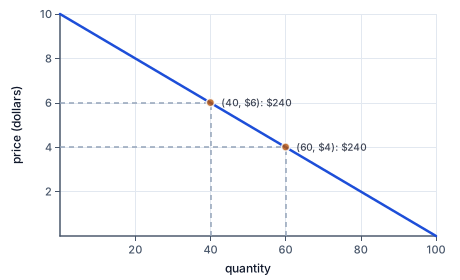
Price in dollars against quantity on a straight demand curve, P = 10 − Q/10. At 4 dollars buyers take 60 units and at 6 dollars 40. Revenue is 4 × 60 = 240 dollars before and 6 × 40 = 240 dollars after: the two rectangles under the points have the same area, and the midpoint elasticity between them is exactly one.

The figure shows the four-to-six-dollar example: the two revenue rectangles have the same 240-dollar area.

Total revenue is price times quantity sold. A price rise pushes revenue upward through the price on each remaining sale but downward through the lost sales. When demand is elastic over the relevant interval, the proportional quantity reduction is larger than the price increase, so revenue falls as price rises. When demand is inelastic, revenue rises with price. With unit midpoint elasticity, the endpoint revenues are equal. These conclusions concern revenue, not profit, because production costs have not yet been deducted.

In the four-to-six-dollar example, initial revenue is four times sixty, or 240 dollars. Final revenue is six times forty, also 240 dollars. Both endpoint totals provide a useful independent check on the elasticity classification. By contrast, if quantity fell from sixty to fifty over the same price change, revenue would rise from 240 to 300 dollars. The smaller proportional quantity response would make demand inelastic over that interval. The revenue comparison should use actual endpoint products rather than adding percentage changes as if their interaction never mattered.

The availability of close substitutes often makes demand more elastic. Consumers can switch away when this good's relative price rises. A narrowly defined brand can therefore have a more elastic demand than a broad category containing many brands. The share of the budget matters too: a large expenditure warrants more adjustment than a tiny one, other things equal. Necessity and habit may reduce responsiveness, although neither label is an infallible numerical rule.

Time can expand the alternatives available. Immediately after an energy-price change, a household's equipment and location are fixed. Over a longer period, it may replace equipment or change travel arrangements. Demand may consequently be more elastic over a longer horizon. Supply responsiveness also depends on time: existing inventories or spare capacity permit a quick response, while building new facilities takes longer. State the horizon in an empirical elasticity claim. A short-run estimate cannot simply be treated as a permanent response for every adjustment period.

Another way: Other elasticities answer different questions

Cross-price elasticity compares the demand for good A with the price of good B. A positive value is consistent with substitutes: when B becomes more expensive, demand for A rises. A negative value is consistent with complements: a higher price of B reduces purchases of A used with it. A value near zero indicates little response in the specified comparison. Keep the goods' roles explicit. An own-price demand elasticity magnitude cannot identify whether two goods are complements.

Income elasticity compares the demand change with an income change, holding other relevant determinants fixed. A positive value identifies a normal good within that model and range. A negative value identifies an inferior good. 'Inferior' is a technical description of the direction of response, not an insult or a statement about physical quality. If income rises ten percent and demand rises fifteen percent, income elasticity is 1.5. If demand instead falls five percent, it is negative 0.5. The sign must be retained to preserve the interpretation.

Supply elasticity measures producers' quantity response to the good's own price. It is usually nonnegative for the standard upward-sloping supply model. The same midpoint procedure can be used over an interval. A steep-looking supply curve is not automatically inelastic without considering its scale and the relevant point. A perfectly inelastic supply is vertical because quantity does not respond to price at all. A perfectly elastic supply is horizontal over the modeled range: suppliers offer the relevant quantities at a given price, as in a stipulated small-country world-supply model.

Elasticity is useful in later analysis of tax burdens. The relatively less responsive side of a market generally bears more of a per-unit tax burden in the standard competitive model. That conclusion depends on behavioral response, not on who is legally assigned to remit the tax. Learning the measure now allows us to explain incidence later rather than memorizing a rule detached from demand and supply.

Finally, distinguish estimation from application. A classroom problem can supply a reliable elasticity and ask for a conditional prediction. A real policy analyst must ask where the estimate came from, what variation identified it, which population it describes and whether the proposed change is within a plausible range. A large extrapolation may invalidate a simple constant-elasticity approximation. The number's apparent precision does not remove uncertainty about the model or its transfer to a new setting.

5. An invented museum's admission experiment

A fictional museum compares two otherwise identical trial periods. At four dollars per ticket it sells sixty tickets; at six dollars it sells forty. The exercise stipulates that exhibits, weather, visitor population and competing attractions remain unchanged. The midpoint quantity change is negative twenty divided by fifty, or negative forty percent. The midpoint price change is two divided by five, or forty percent. The magnitude of demand elasticity is one, and revenue is 240 dollars in either period.

This result does not tell the museum which price maximizes profit. If admitting each additional visitor costs one dollar, variable costs are sixty dollars in the first period and forty in the second. The same revenue then corresponds to different contributions toward fixed costs. Nor does revenue determine which admission policy best meets an access objective. The museum may care about participation by different groups, educational benefits or funding conditions. Those questions need additional evidence and explicit objectives.

Suppose a nearby alternative attraction later raises its admission price by ten percent, while demand for the museum rises by five percent with the museum's own price unchanged. Under the supplied causal comparison, the museum's cross-price elasticity with respect to that attraction is positive 0.5. That suggests substitution over this range. It is not the museum's own-price elasticity and cannot replace it in the earlier calculation.

In a real trial the 'otherwise identical' assumption would need scrutiny. A special exhibition coinciding with the higher price could conceal a negative own-price effect. Recording only two prices and two sales totals would not separate the exhibition shift from the price response. The exercise therefore teaches both a calculation and the conditions required to interpret it as responsiveness along a stable demand schedule.

6. Check the tempting shortcut

Elasticity is not the same as slope. Use average bases for both midpoint changes, retain cross-price and income signs, and distinguish revenue from profit. A before-and-after ratio does not isolate a price effect when other demand determinants changed.

7. In the fictional Alder model, quantity demanded changes from 60 to 40 when price rises from 4 to 6 dollars, with other demand determinants fixed. In a separate comparison, income rises 10 percent and demand for a different good rises 15 percent. Calculate the magnitude of the first good's midpoint price elasticity, its initial revenue in dollars, and the second good's income elasticity.

8. In the fictional Birch model, quantity demanded changes from 120 to 80 when price rises from 8 to 12 dollars, with other demand determinants fixed. In a separate comparison, income rises 10 percent and demand for a different good rises 15 percent. Calculate the magnitude of the first good's midpoint price elasticity, its initial revenue in dollars, and the second good's income elasticity.

9. In the fictional Cedar model, quantity demanded changes from 180 to 120 when price rises from 12 to 18 dollars, with other demand determinants fixed. In a separate comparison, income rises 10 percent and demand for a different good rises 15 percent. Calculate the magnitude of the first good's midpoint price elasticity, its initial revenue in dollars, and the second good's income elasticity.

10. In the fictional Dune model, quantity demanded changes from 240 to 160 when price rises from 16 to 24 dollars, with other demand determinants fixed. In a separate comparison, income rises 10 percent and demand for a different good rises 15 percent. Calculate the magnitude of the first good's midpoint price elasticity, its initial revenue in dollars, and the second good's income elasticity.

11. Guided practice

In the fictional Elm model, quantity demanded changes from 300 to 200 when price rises from 20 to 30 dollars, with other demand determinants fixed. In a separate comparison, income rises 10 percent and demand for a different good rises 15 percent. Calculate the magnitude of the first good's midpoint price elasticity, its initial revenue in dollars, and the second good's income elasticity.

12. Guided practice

In the fictional Dune model, quantity demanded changes from 240 to 160 when price rises from 16 to 24 dollars, with other demand determinants fixed. In a separate comparison, income rises 10 percent and demand for a different good rises 15 percent. Calculate the magnitude of the first good's midpoint price elasticity, its initial revenue in dollars, and the second good's income elasticity.

13. Guided practice

In the fictional Fern model, quantity demanded changes from 360 to 240 when price rises from 24 to 36 dollars, with other demand determinants fixed. In a separate comparison, income rises 10 percent and demand for a different good rises 15 percent. Calculate the magnitude of the first good's midpoint price elasticity, its initial revenue in dollars, and the second good's income elasticity.

14. Practice

In the fictional Grove model, quantity demanded changes from 420 to 280 when price rises from 28 to 42 dollars, with other demand determinants fixed. In a separate comparison, income rises 10 percent and demand for a different good rises 15 percent. Calculate the magnitude of the first good's midpoint price elasticity, its initial revenue in dollars, and the second good's income elasticity.

15. Practice

With other determinants fixed, the price of good B rises 10 percent and demand for good A falls 5 percent. Separately, income rises 8 percent and demand for good C rises 12 percent. A supplied supply comparison has a 10 percent price rise and a 20 percent quantity-supplied rise. Calculate the signed cross-price elasticity of A with respect to B, the income elasticity of C, and the supply elasticity. Use these supplied percentages, not new midpoint bases.

16. Somewhere new

A museum compares two admission trials with unchanged exhibits and visitor population, and separately studies an income change affecting another service. Its report needs a responsiveness measure and a revenue check, not a claim about profit or a universal demand parameter. In the fictional Island model, quantity demanded changes from 540 to 360 when price rises from 36 to 54 dollars, with other demand determinants fixed. In a separate comparison, income rises 10 percent and demand for a different good rises 15 percent. Calculate the magnitude of the first good's midpoint price elasticity, its initial revenue in dollars, and the second good's income elasticity.

17. Lesson test

Lesson test: one question per skill, one attempt each, no hints. Your answers are checked when you submit.

18. Test question

In the fictional Juniper model, quantity demanded changes from 600 to 400 when price rises from 40 to 60 dollars, with other demand determinants fixed. In a separate comparison, income rises 10 percent and demand for a different good rises 15 percent. Calculate the magnitude of the first good's midpoint price elasticity, its initial revenue in dollars, and the second good's income elasticity.

19. What you can do now

Reconstruct the model without the worked example. Explain each requested measure's units and identify an assumption that the conclusion depends on.

Working for the steps left to you

	Calculated value
Midpoint elasticity magnitude
Initial revenue
Income elasticity

	Calculated value
Midpoint elasticity magnitude
Initial revenue
Income elasticity

	Calculated value
Midpoint elasticity magnitude
Initial revenue
Income elasticity