Price discrimination and the allocation of surplus

Paper packet. Every task here also exists on screen, where it is checked automatically; answers written on paper are not assessed by Nydus. When you are back at a device, enter your answers there.

1. What you will learn

Analyze price discrimination and the allocation of surplus using explicit assumptions, calculated results and a stated limit of the model.

2. Starting point

A single-price monopolist lowers the price on earlier units when it expands sales, so marginal revenue is below price. Total surplus adds buyers' and sellers' gains, while distribution records who receives them. Efficient output need not imply a fair division.

3. Terms and units

4. Different prices require an economic explanation

A seller sometimes charges different buyers different effective prices for the same or closely comparable product. The difference is price discrimination when it is not fully explained by different costs of serving those buyers. A higher delivery charge for a remote destination may simply reflect higher transport cost. A discount to one group with the same delivery cost may instead reflect a pricing strategy based on willingness to pay or responsiveness. The classification requires information about costs and conditions, not just two different price tags.

Successful discrimination generally requires some market power, a way to distinguish buyers or induce them to select different terms, and limits on resale. If anyone can buy cheaply and resell freely to high-price buyers, the proposed price gap creates an arbitrage opportunity. The lower-price purchases then compete with the seller's higher-price offer. Tickets tied to named users, nontransferable services or different contract conditions can limit resale in real arrangements, although those arrangements can have their own costs and legal constraints.

Information matters. A seller rarely knows each buyer's exact willingness to pay. It may observe a group characteristic, purchasing history, time of purchase or the package a buyer selects. These signals are imperfect. A classroom model can stipulate exact values to isolate the pricing logic, but that assumption should not be mistaken for a claim about what businesses actually know. Administrative effort, mistaken classification and privacy concerns are outside a simple revenue table unless explicitly included.

Price discrimination is therefore a family of strategies rather than a single universal outcome. Some expand output relative to single-price monopoly, some mostly redistribute surplus and some can reduce access for particular groups. The welfare conclusion depends on the form, the counterfactual and the cost of implementing it. A useful analysis begins by naming the specific pricing rule and the feasible purchases under that rule.

Term	What it means
Price discrimination	Charging different effective prices for comparable units for reasons not fully explained by differences in provision cost.
First-degree discrimination	Charging each buyer the maximum willingness to pay for each purchased unit in the idealized model.
Market segmentation	Separating buyers into groups facing different prices or terms.
Self-selection	Buyers choosing among offered packages or contracts in ways that reveal information about their preferences.
Arbitrage	Buying in a lower-price market and reselling in a higher-price market.
Consumer surplus	The gap between willingness to pay and the actual payment on purchased units.

Another way: Perfect first-degree discrimination is an informative limit

Consider four buyers who each want at most one unit and value it at twelve, ten, eight and six dollars. Marginal cost is five dollars for every unit and fixed cost is zero. Under ideal first-degree discrimination, the seller knows each value and can charge each buyer exactly that amount. Resale is impossible and each buyer accepts a purchase at equality under the supplied convention. All four values exceed cost, so all four trades can create positive gains.

Revenue is twelve plus ten plus eight plus six, or thirty-six dollars. Variable cost is four times five, or twenty. Producer surplus is sixteen. Each buyer pays exactly the corresponding willingness to pay, leaving zero consumer surplus. Total surplus is nevertheless sixteen because every listed beneficial trade occurs. In this idealized case, the seller captures all the modeled gains rather than leaving them with buyers.

The output can be efficient even though the distribution strongly favors the seller. The seller can serve an additional low-value buyer without reducing the prices charged to earlier buyers. It therefore accepts every unit whose willingness to pay exceeds marginal cost. In a continuous version, the last unit satisfies demand equal to marginal cost rather than the single-price marginal-revenue condition. The private incentive to add units aligns with the basic gain-from-trade condition because earlier payments need not fall.

That result rests on demanding assumptions: exact knowledge, enforceable individualized payments, no resale, no implementation cost and the stated acceptance rule at equality. If buyers can conceal their values or refuse a zero-surplus offer for reasons outside the model, the seller cannot simply extract the calculated amount. The model is a benchmark demonstrating how price uniformity affects output incentives, not a prediction that actual sellers routinely achieve perfect extraction.

Another way: Compare with a single price using the same buyers

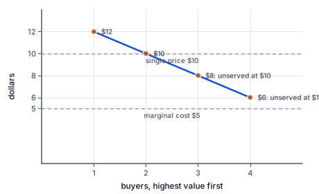
Each buyer's value in dollars, highest first: 12, 10, 8 and 6, with a marginal cost of 5 dollars for every unit. The best single price, 10 dollars, sells two units and leaves the 8-dollar and 6-dollar buyers unserved although their values exceed the 5-dollar cost. Charging each buyer their own value serves all four.

The figure shows the four buyers' values against the single price and the marginal cost: two buyers worth serving are left out at ten dollars.

For the same four buyers, a single price of twelve sells one unit and produces profit of seven dollars. A price of ten sells two, giving revenue twenty and cost ten, so profit is ten. A price of eight sells three, giving revenue twenty-four and cost fifteen, so profit is nine. A price of six sells four, giving revenue twenty-four and cost twenty, so profit is four. The best listed single price is ten, selling two units.

At that single-price outcome, consumer surplus is two dollars: the twelve-dollar buyer pays ten, while the ten-dollar buyer has zero surplus under the equality convention. Producer surplus and profit are ten because fixed cost is zero. Total surplus is twelve. The omitted buyers with values eight and six would create gains of three and one respectively if served at the five-dollar marginal cost. Their four dollars of unrealized gains are the deadweight loss relative to serving all four.

Moving to perfect first-degree discrimination raises output from two to four and total surplus from twelve to sixteen in this particular model. Producer surplus rises from ten to sixteen, while consumer surplus falls from two to zero. Part of the seller's gain is a transfer of the original buyers' surplus; another part comes from gains on newly served buyers. Reporting only the higher total or only the lower consumer surplus would omit an important dimension of the comparison.

This method of comparison is broadly useful: hold demand values and costs fixed, specify both pricing regimes, solve each feasible choice and compare quantities and surplus accounts. Do not compare an individualized-price example with a different single-price market and attribute every difference to discrimination. A valid counterfactual changes the pricing rule while keeping the other relevant conditions consistent.

Another way: Segmentation and self-selection have different limits

A seller may divide buyers into groups and set a separate uniform price in each. If marginal cost is common and the groups cannot resell, profit maximization compares marginal revenue in each served group with that common marginal cost. Under the standard conditions, the group with relatively less elastic demand at the chosen prices pays the higher markup. This is a responsiveness comparison, not a rule that every observed demographic group has a fixed or universal elasticity.

Group pricing does not guarantee efficient output. Each group's uniform price can still restrict sales within that group. Relative to a single common price, one group's output may rise while another's falls. The total output and surplus effects require calculation. The perfect first-degree result cannot be transferred automatically to this less informative setting. A policy assessment must also distinguish the efficiency calculation from distributional or legal questions about which classifications may be used.

Second-degree forms use menus, such as quantity packages or versions with different features, that buyers choose for themselves. A seller may not know an individual's valuation beforehand but can design options that appeal differently to high- and low-demand buyers. A buyer's choice reveals something about preferences. Designing such a menu requires respecting incentive compatibility: a high-value buyer must not prefer the option intended for low-value buyers if the seller's predicted segmentation is to occur.

A two-part tariff charges an access fee plus a per-unit usage price. If usage price equals marginal cost, participating buyers face an efficient marginal consumption incentive under the basic model. The fixed fee can capture some surplus or finance fixed cost. But a high fee can deter participation, especially when buyers have different demands. Thus efficient use by those who join does not prove efficient access for the whole population. Both margins need analysis.

Discounts tied to timing or restrictions can also screen buyers. A flexible advance purchaser may accept a lower-price but less adaptable arrangement, while someone needing flexibility pays more. The effective product includes those terms, so any interpretation must examine their costs and value. A lower nominal price alone is not enough to identify whether the seller is reducing cost, segmenting demand or both.

In every case, the report should distinguish the seller's objective from the evaluator's criterion. A profit-maximizing pricing strategy need not maximize consumer surplus, total surplus or access. The lesson's constructed tasks grade the result under a supplied rule; they do not ask the learner to endorse that rule. Stating the counterfactual and the information assumptions makes the conclusion both precise and appropriately limited.

Another way: State the participation convention

If a buyer pays exactly the maximum willingness to pay, the buyer is indifferent between purchasing and not purchasing in the numerical model. Perfect-extraction examples conventionally specify acceptance at equality, or interpret the charge as arbitrarily slightly below that value. Our discrete cases use acceptance at equality. Without a convention, exact sales at reservation values can be ambiguous even though the potential gains from trade are clear.

5. Four seats in a fictional demonstration

An invented demonstration has four potential participants with values of twelve, ten, eight and six dollars for one seat each. Providing each seat costs five dollars, and there is no fixed cost. A single uniform price of ten dollars is the most profitable among the candidate prices equal to those values: two seats sell and profit is ten dollars. The two excluded participants would still value attendance above its cost, but lowering the common price enough to include them reduces receipts from earlier buyers.

Now stipulate an ideal individualized system: the organizer knows each value, charges exactly that value and prevents transfers of admission rights. Four seats sell, revenue is thirty-six dollars and profit is sixteen. Consumer surplus is zero. The new allocation includes every beneficial trade, but the participants do not retain the surplus they would have received under a lower uniform price. Calling the result simply 'better' would omit the criterion being used.

The organizer cannot infer that an actual personalized offer will reproduce those numbers. Participants may conceal preferences, share access or decline terms, and administering the system may cost resources. If the organizer instead offers a discounted group price based on an imperfect observable characteristic, the first-degree calculation no longer applies. A fresh demand and cost comparison is needed.

An audit should therefore list output, payments, producer surplus, consumer surplus and the information required for each regime. It can then ask whether the institution values total gains, participant access, a particular distribution or another objective. The numerical exercise illuminates the trade-offs without turning an idealized profit calculation into a universal recommendation for how real events should charge.

6. Check the tempting shortcut

Not every price difference is discrimination; costs and contract terms matter. Perfect first-degree discrimination can yield efficient output while leaving buyers no surplus, but its result does not automatically apply to group pricing or menus. Compare regimes using the same underlying values and costs.

7. In the fictional Alder model, four buyers each want at most one unit and value it at [13, 11, 9, 7] dollars respectively. A seller has constant marginal cost 6 dollars and no fixed cost. Under perfect first-degree price discrimination, values are known and resale is impossible; each buyer pays exactly that buyer's value. Calculate units sold, total revenue, and producer surplus in dollars.

8. In the fictional Birch model, four buyers each want at most one unit and value it at [14, 12, 10, 8] dollars respectively. A seller has constant marginal cost 7 dollars and no fixed cost. Under perfect first-degree price discrimination, values are known and resale is impossible; each buyer pays exactly that buyer's value. Calculate units sold, total revenue, and producer surplus in dollars.

9. In the fictional Cedar model, four buyers each want at most one unit and value it at [15, 13, 11, 9] dollars respectively. A seller has constant marginal cost 8 dollars and no fixed cost. Under perfect first-degree price discrimination, values are known and resale is impossible; each buyer pays exactly that buyer's value. Calculate units sold, total revenue, and producer surplus in dollars.

10. In the fictional Dune model, four buyers each want at most one unit and value it at [16, 14, 12, 10] dollars respectively. A seller has constant marginal cost 9 dollars and no fixed cost. Under perfect first-degree price discrimination, values are known and resale is impossible; each buyer pays exactly that buyer's value. Calculate units sold, total revenue, and producer surplus in dollars.

11. Guided practice

In the fictional Elm model, four buyers each want at most one unit and value it at [17, 15, 13, 11] dollars respectively. A seller has constant marginal cost 10 dollars and no fixed cost. Under perfect first-degree price discrimination, values are known and resale is impossible; each buyer pays exactly that buyer's value. Calculate units sold, total revenue, and producer surplus in dollars.

12. Guided practice

In the fictional Dune model, four buyers each want at most one unit and value it at [16, 14, 12, 10] dollars respectively. A seller has constant marginal cost 9 dollars and no fixed cost. Under perfect first-degree price discrimination, values are known and resale is impossible; each buyer pays exactly that buyer's value. Calculate units sold, total revenue, and producer surplus in dollars.

13. Guided practice

In the fictional Fern model, four buyers each want at most one unit and value it at [18, 16, 14, 12] dollars respectively. A seller has constant marginal cost 11 dollars and no fixed cost. Under perfect first-degree price discrimination, values are known and resale is impossible; each buyer pays exactly that buyer's value. Calculate units sold, total revenue, and producer surplus in dollars.

14. Practice

In the fictional Grove model, four buyers each want at most one unit and value it at [19, 17, 15, 13] dollars respectively. A seller has constant marginal cost 12 dollars and no fixed cost. Under perfect first-degree price discrimination, values are known and resale is impossible; each buyer pays exactly that buyer's value. Calculate units sold, total revenue, and producer surplus in dollars.

15. Practice

Four buyers value one unit each at 12,10,8,6 dollars. Constant marginal cost is 5 dollars and fixed cost is zero. Unlike the individualized-price examples, the seller must choose one common price from 12,10,8,6. Buyers purchase at equality. Calculate the profit-maximizing common price, units sold, and economic profit.

16. Somewhere new

An organizer can identify four visitors' reservation values and issues nontransferable, individually priced admission rights. Compare receipts with provision cost under that idealized rule, without treating the resulting division of gains as an endorsement of the pricing policy. In the fictional Island model, four buyers each want at most one unit and value it at [21, 19, 17, 15] dollars respectively. A seller has constant marginal cost 14 dollars and no fixed cost. Under perfect first-degree price discrimination, values are known and resale is impossible; each buyer pays exactly that buyer's value. Calculate units sold, total revenue, and producer surplus in dollars.

17. Lesson test

Lesson test: one question per skill, one attempt each, no hints. Your answers are checked when you submit.

18. Test question

In the fictional Juniper model, four buyers each want at most one unit and value it at [22, 20, 18, 16] dollars respectively. A seller has constant marginal cost 15 dollars and no fixed cost. Under perfect first-degree price discrimination, values are known and resale is impossible; each buyer pays exactly that buyer's value. Calculate units sold, total revenue, and producer surplus in dollars.

19. What you can do now

Reconstruct the model without the worked example. Explain each requested measure's units and identify an assumption that the conclusion depends on.

Working for the steps left to you

	Constructed result
Common price
Units sold
Profit