Short-run costs and long-run scale

Paper packet. Every task here also exists on screen, where it is checked automatically; answers written on paper are not assessed by Nydus. When you are back at a device, enter your answers there.

1. What you will learn

Analyze short-run costs and long-run scale using explicit assumptions, calculated results and a stated limit of the model.

2. Starting point

Production uses inputs with opportunity costs. Total product, marginal product and average product describe different physical measures. In the short run at least one input is fixed; in the long run all inputs can be varied.

3. Terms and units

4. Classify costs relative to the decision

A cost is fixed when it does not change with the output choice over the relevant range and period. A workshop's lease payment might be fixed for the current month. Materials used per unit and labor hours that can be adjusted with production may be variable. The classification depends on the decision. Over a longer horizon the workshop may choose a different building or end the lease, so a currently fixed cost need not remain unavoidable forever.

Fixed and sunk are related but distinct terms. A fixed cost does not vary with output within the stated range. A sunk cost has already been incurred and cannot be recovered. A future fixed fee that can be avoided by exiting before a contract begins is not sunk at that decision point. A machine already purchased might have a resale value, making part of its historical expenditure recoverable. Identify which alternatives change a cost rather than assigning categories solely from the expense's name.

Economic cost includes opportunity costs, including implicit costs that do not appear as an explicit payment. Using an owner-provided room can forgo rental income. The owner's time can forgo earnings elsewhere. Accounting records may omit those forgone alternatives, but economic-profit analysis includes them when they are relevant. A numerical problem should state whether its costs already include all opportunity costs; otherwise subtracting an implicit cost twice would be as wrong as omitting it.

Total cost is fixed cost plus variable cost at a specified output: TC = FC + VC. Every amount must refer to the same period and output. If fixed cost is forty dollars for a day and variable cost at ten units is sixty dollars for that day, total cost is one hundred. Combining a monthly lease with one day's materials without conversion would not provide a valid daily total. Units are part of the economic model, not decoration around the arithmetic.

Term	What it means
Fixed cost	A cost that does not vary with output over the stated short-run decision range.
Variable cost	A cost that changes with output over that range.
Average total cost	Total economic cost divided by output.
Average variable cost	Variable cost divided by output.
Marginal cost	The change in total cost divided by the change in output.
Economies of scale	A range in which long-run average cost falls as output expands.
Diseconomies of scale	A range in which long-run average cost rises as output expands.

Another way: Averages divide totals; margins compare alternatives

Average fixed cost is FC/Q, average variable cost is VC/Q and average total cost is TC/Q for positive output. Since TC = FC + VC, average total cost equals average fixed cost plus average variable cost. In the forty-dollar fixed-cost and sixty-dollar variable-cost example at ten units, AFC is four, AVC is six and ATC is ten dollars per unit. These three averages answer different questions and should not be substituted for one another.

Marginal cost compares two output levels. If variable cost rises from sixty to sixty-nine dollars when output rises from ten to eleven, while fixed cost stays forty, total cost rises from one hundred to one hundred nine. The extra unit costs nine dollars. MC is nine, below the initial ATC of ten but above the initial AVC of six. There is no contradiction: the three numbers use different numerators and denominators.

If output increases by more than one unit, divide the cost change by the output change. A total-cost increase of twenty dollars for four extra units implies an average marginal cost of five dollars per unit over that interval. It does not establish that each of the four units individually costs five unless additional assumptions are supplied. A coarse table reveals an interval comparison; a finer table or function is required for unit-by-unit increments.

At zero output, average costs are undefined because Q is zero. Total fixed cost may still be positive, and variable cost may be zero under the standard shutdown assumption. Do not assign a zero ATC to a firm that produces nothing; there are no units over which to spread the cost. Marginal cost of the first unit can still be calculated by comparing total costs at zero and one. The distinction mirrors the difference between total and average product at zero labor.

Another way: Read short-run curves through their arithmetic

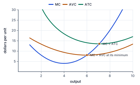
Dollars per unit against output for a firm with variable cost Q³/3 − 4Q² + 20Q and a fixed cost of 36. Marginal cost falls to its lowest at 4 units and then rises. It crosses average variable cost at that curve's minimum, 8 dollars at 6 units, and average total cost at its minimum, about 13.5 dollars near 7.1 units. The gap between the two averages is average fixed cost, which narrows as output grows.

The figure draws a smooth set of short-run curves: marginal cost crosses each average at that average's lowest point.

Average fixed cost falls as positive output rises because an unchanged amount is spread over more units. That decline alone does not imply that every other cost measure falls. Average variable cost may first fall and then rise as specialization gives way to diminishing marginal returns. Average total cost combines those patterns. Its downward portion can reflect both falling AVC and the spreading of fixed cost; later a rising AVC may outweigh the continued decline in AFC.

When marginal cost is below an existing average, an additional unit lowers that average. When marginal cost is above the average, the additional unit raises it. If the added unit costs exactly the old average, the average is unchanged. The relevant average must be named: MC can be above AVC while below ATC, raising the former and lowering the latter at the same output transition.

In a smooth conventional cost diagram, MC crosses AVC at AVC's minimum and ATC at ATC's minimum. A discrete table need not display an exact equality in a listed row, because its increments span intervals. Calculate the data before applying the visual rule. The gap between ATC and AVC at any positive quantity is AFC, and that gap narrows as output rises when fixed cost is constant. The curves do not become identical at a finite output merely because the gap is smaller.

The production relationship explains part of the pattern. With a fixed wage and labor as the only variable input, higher marginal product means less extra labor cost per unit of extra output. As marginal product falls, marginal cost rises. This is a short-run relationship with fixed capital. A technological improvement, lower input price or change in the fixed input can shift the cost curves, rather than cause a movement along an unchanged curve.

An increase in fixed cost alone raises TC and ATC but leaves VC, AVC and MC unchanged under the stated assumptions. An increase in a variable input price generally raises variable and marginal costs. Distinguishing those effects is useful for output decisions: a sunk fixed-cost increase cannot make an already worthwhile marginal unit cease to cover its marginal cost, although it can alter total profit and the desirability of remaining in the industry over a longer horizon.

Another way: Choose plant size in the long run

In the long run, the producer can choose all inputs, including plant size. Long-run average cost records the lowest attainable average cost for each output when those choices can be adjusted. It can be represented as the lower envelope of the available short-run average-cost curves. For a small output, a small plant may be cheapest; for a larger output, a larger plant may become economical. The firm is not required to use the same plant at every output in the long-run comparison.

Economies of scale occur where long-run average cost decreases as output expands. Possible mechanisms include specialization, spreading certain indivisible facilities over more output and engineering relationships that make larger systems cheaper per unit. Constant returns in cost terms describe a flat long-run average-cost range, while diseconomies of scale describe a rising range. Coordination, communication or management difficulties can contribute to the latter. These are possible mechanisms, not assumptions that every industry has an identical U-shaped long-run curve.

Returns to scale is a technological concept: how output responds when all inputs increase proportionately. Economies of scale is a cost concept: how minimum average cost responds to output. With unchanged input prices and appropriate production conditions, increasing returns to scale can generate economies of scale. Changing input prices or purchasing conditions can also affect costs, so the terms should not be treated as interchangeable in every setting. State whether the comparison concerns physical input-output ratios or monetary cost.

Minimum efficient scale is the smallest output at which the lowest long-run average cost is reached, when such a range exists. If it is large relative to total market demand, a market may support only a few low-cost producers. If it is small relative to demand, many firms may operate efficiently. This connection helps explain why cost conditions matter for market structure, but the conclusion also depends on entry conditions, product differentiation and the size of demand.

Do not identify falling short-run ATC caused by spreading an existing fixed cost as proof of long-run economies of scale. The former holds a plant fixed; the latter permits all inputs to change. Likewise, diminishing marginal returns to labor with capital fixed does not prove diseconomies of scale when labor and capital expand together. The safest approach is to describe the experiment first: which inputs can change, which prices are held fixed, and what output range is being compared? Only then attach the appropriate cost label.

5. A fictional printing workshop compares two choices

A printing workshop has a forty-dollar daily fixed commitment and incurs sixty dollars of variable cost for ten print batches. Total cost is one hundred dollars, ATC is ten and AVC is six dollars per batch. An eleventh batch raises variable cost to sixty-nine. Its marginal cost is nine dollars. Because nine is below the old ATC, the new ATC falls to one hundred nine divided by eleven, even though AVC rises to sixty-nine divided by eleven. This single increment illustrates why averages must be named precisely.

The owner next receives a notice that an unavoidable daily fixed fee rises by twenty dollars. At the same production quantities, total cost and average total cost increase, but the extra variable cost of the eleventh batch remains nine. A decision about that batch should compare its additional revenue with nine, not with the entire new fixed fee. A separate decision about renewing the business arrangement for a future period should consider costs that can then be avoided.

Finally, the owner considers replacing the small press with a larger one. The original cost table does not describe that new equipment configuration. A long-run comparison requires the larger press's total and average costs at relevant outputs. It might be cheaper for a high-volume operation but more expensive at ten batches. Calling it 'more efficient' without specifying output would obscure the choice.

The resulting report has three distinct comparisons: an extra batch with the same press, a fixed-fee change with the same technology, and a plant-size choice. Keeping those comparisons separate prevents the owner from mistaking a short-run average-cost movement for a technological improvement or a long-run economy of scale. All numbers are classroom assumptions, not a recommendation for a real printing business.

6. Check the tempting shortcut

Average total cost is not marginal cost, and an unavoidable fixed payment is not added to every unit's marginal cost. Falling ATC from spreading a fixed cost does not by itself demonstrate long-run economies of scale. The short-run and long-run experiments allow different inputs to change.

7. In the fictional Alder model, a firm's fixed cost is 40 dollars and variable cost at 10 units is 60 dollars. Increasing output to 11 units raises variable cost to 69 dollars; fixed cost does not change. Calculate average total cost at 10, average variable cost there, and marginal cost of the extra unit. All figures cover the same day.

8. In the fictional Birch model, a firm's fixed cost is 80 dollars and variable cost at 20 units is 120 dollars. Increasing output to 21 units raises variable cost to 129 dollars; fixed cost does not change. Calculate average total cost at 20, average variable cost there, and marginal cost of the extra unit. All figures cover the same day.

9. In the fictional Cedar model, a firm's fixed cost is 120 dollars and variable cost at 30 units is 180 dollars. Increasing output to 31 units raises variable cost to 189 dollars; fixed cost does not change. Calculate average total cost at 30, average variable cost there, and marginal cost of the extra unit. All figures cover the same day.

10. In the fictional Dune model, a firm's fixed cost is 160 dollars and variable cost at 40 units is 240 dollars. Increasing output to 41 units raises variable cost to 249 dollars; fixed cost does not change. Calculate average total cost at 40, average variable cost there, and marginal cost of the extra unit. All figures cover the same day.

11. Guided practice

In the fictional Elm model, a firm's fixed cost is 200 dollars and variable cost at 50 units is 300 dollars. Increasing output to 51 units raises variable cost to 309 dollars; fixed cost does not change. Calculate average total cost at 50, average variable cost there, and marginal cost of the extra unit. All figures cover the same day.

12. Guided practice

In the fictional Dune model, a firm's fixed cost is 160 dollars and variable cost at 40 units is 240 dollars. Increasing output to 41 units raises variable cost to 249 dollars; fixed cost does not change. Calculate average total cost at 40, average variable cost there, and marginal cost of the extra unit. All figures cover the same day.

13. Guided practice

In the fictional Fern model, a firm's fixed cost is 240 dollars and variable cost at 60 units is 360 dollars. Increasing output to 61 units raises variable cost to 369 dollars; fixed cost does not change. Calculate average total cost at 60, average variable cost there, and marginal cost of the extra unit. All figures cover the same day.

14. Practice

In the fictional Grove model, a firm's fixed cost is 280 dollars and variable cost at 70 units is 420 dollars. Increasing output to 71 units raises variable cost to 429 dollars; fixed cost does not change. Calculate average total cost at 70, average variable cost there, and marginal cost of the extra unit. All figures cover the same day.

15. Practice

A firm produces q positive units, incurs fixed cost f dollars and variable cost v dollars. Construct average total cost using f,v,q.

16. Somewhere new

A printing workshop receives a request for one additional batch using its existing press. Its accountant supplies total cost categories and the extra materials-and-labor bill. Keep the current average costs separate from the cost of accepting that additional batch. In the fictional Island model, a firm's fixed cost is 360 dollars and variable cost at 90 units is 540 dollars. Increasing output to 91 units raises variable cost to 549 dollars; fixed cost does not change. Calculate average total cost at 90, average variable cost there, and marginal cost of the extra unit. All figures cover the same day.

17. Lesson test

Lesson test: one question per skill, one attempt each, no hints. Your answers are checked when you submit.

18. Test question

In the fictional Juniper model, a firm's fixed cost is 400 dollars and variable cost at 100 units is 600 dollars. Increasing output to 101 units raises variable cost to 609 dollars; fixed cost does not change. Calculate average total cost at 100, average variable cost there, and marginal cost of the extra unit. All figures cover the same day.

19. What you can do now

Reconstruct the model without the worked example. Explain each requested measure's units and identify an assumption that the conclusion depends on.

Working for the steps left to you