Tax wedges, incidence and deadweight loss

Paper packet. Every task here also exists on screen, where it is checked automatically; answers written on paper are not assessed by Nydus. When you are back at a device, enter your answers there.

1. What you will learn

Analyze tax wedges, incidence and deadweight loss using explicit assumptions, calculated results and a stated limit of the model.

2. Starting point

Competitive equilibrium sets buyers' willingness to pay equal to sellers' marginal cost. Consumer and producer surplus measure gains from completed trades. A transfer changes who receives an amount; deadweight loss concerns gains no participant receives.

3. Terms and units

4. One transaction, two relevant prices

Without a tax, a buyer's payment and a seller's receipt are the same price in the basic competitive model. A per-unit tax separates them. If the buyer pays fourteen dollars and the seller retains ten after a four-dollar tax, the wedge is fourteen minus ten, or four. Denote the buyer price Pb and the seller price Ps. The accounting condition is Pb - Ps = t, where t is the tax per unit. This condition must hold alongside the demand and supply relationships.

Demand is evaluated at the amount buyers actually pay. Supply is evaluated at the amount sellers actually retain. Using the buyer price in both schedules would pretend sellers keep money remitted as tax. Using the seller receipt in both would pretend buyers do not pay the tax. The two-price notation prevents that mistake. Quantity demanded at Pb must equal quantity supplied at Ps, while the two prices differ by the wedge.

The law may require sellers to remit the tax or require buyers to pay it separately. In the standard competitive model with the same enforcement and no additional transaction costs, these collection arrangements lead to the same economic allocation. If sellers remit, a supply curve drawn in terms of the gross buyer price shifts upward by the tax. If buyers remit, a demand curve drawn in terms of the seller's net receipt shifts downward. Both diagrams express the same relationship between the two relevant prices.

That equivalence is a model result with conditions. Actual administrative rules can affect compliance costs, salience, evasion or timing. If those differ, the policies need not be economically identical. The introductory incidence calculation holds them fixed. It asks how price and quantity adjust to a given wedge, not whether every conceivable method of collecting a tax has identical practical consequences.

Term	What it means
Per-unit tax	A fixed tax amount collected for each unit exchanged.
Tax wedge	The difference between the price buyers pay and the amount sellers retain.
Statutory incidence	The party legally responsible for remitting a tax.
Economic incidence	How a tax changes buyers' payments and sellers' receipts relative to the no-tax benchmark.
Tax revenue	Tax per unit multiplied by the quantity actually taxed.
Deadweight loss of a tax	The foregone gains from trades prevented by the tax in the stated no-externality benchmark.

Another way: Solve the wedge rather than guessing who pays

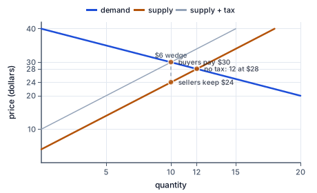
Price in dollars against quantity. Demand Pb = 40 − Q and supply Ps = 4 + 2Q cross at 12 units and 28 dollars before the tax. A tax of 6 dollars a unit opens a wedge: at 10 units buyers pay 30 dollars and sellers keep 24. Buyers pay 2 dollars more and sellers 4 dollars less, so sellers bear two thirds of this tax.

The figure draws this example: the six-dollar wedge between the buyer price and the seller price at ten units.

Use inverse demand Pb = 40 - Q and inverse supply Ps = 4 + 2Q. Before a tax, their equality gives 40 - Q = 4 + 2Q, so quantity is twelve. The shared price is twenty-eight dollars. This no-tax outcome is the benchmark for incidence. Without it, a statement such as 'buyers pay thirty dollars' does not reveal how much the tax increased their payment.

Introduce a tax of six dollars per unit. Substitute both schedules into Pb - Ps = 6: (40 - Q) - (4 + 2Q) = 6. Simplifying gives 36 - 3Q = 6, hence Q = 10. The buyer price is 40 - 10 = 30 dollars. The seller receipt is 4 + 2 times 10 = 24 dollars. The difference is six, so the wedge condition checks correctly.

Relative to the original twenty-eight-dollar price, buyers pay two dollars more and sellers retain four dollars less. Those two changes sum to the six-dollar tax. Buyers bear one third of the per-unit burden and sellers bear two thirds in this model. The tax's statutory assignment was not needed for that calculation. The burden is determined by how the two sides adjust along their schedules.

It is useful to solve in a consistent order: identify the no-tax benchmark, write the wedge, find the taxed quantity, recover both prices, and compare each with the benchmark. Starting with an unsupported assumption that each side bears half can produce plausible-looking numbers that do not satisfy demand or supply. Equal division occurs only for particular responsiveness relationships, not because there are two parties to a transaction.

Another way: Relative responsiveness explains the burden

The side less able or willing to reduce quantity in response to an unfavorable price tends to bear more of the tax in the standard model. If buyers can readily switch to close substitutes while sellers have specialized resources with few alternative uses, sellers may need to absorb more of the wedge to preserve transactions. If buyers have few substitutes while production can easily shift elsewhere, buyers may bear more. This is a comparison of responsiveness on both sides, not a description of which side is morally responsible.

Elasticities express that responsiveness in proportional terms. In a local competitive analysis, relatively inelastic demand places more burden on buyers, while relatively inelastic supply places more on sellers. Comparing raw slopes from graphs with different units can be misleading. Within a single specified market and consistent units, the shapes help illustrate the mechanism; elasticity clarifies the proportional comparison.

Extreme cases make the logic visible. With perfectly inelastic supply, quantity is fixed over the modeled range. A per-unit tax can reduce sellers' receipts without reducing the traded quantity, so sellers bear the burden under the usual demand conditions. With perfectly inelastic demand, buyers continue to demand the fixed quantity and bear the wedge through a higher gross price, assuming supply can provide it. A perfectly elastic side cannot sustain a less favorable net price in the model, shifting the burden to the other side.

Time matters because substitution possibilities can change. A short-run burden may differ from a long-run burden when households replace equipment, firms enter or exit, or resources move between uses. A statement about incidence should name the horizon and the maintained assumptions. The numerical exercise supplies fixed schedules, so its answer is exact within those schedules. It is not a prediction that any real tax with the same statutory rate will have the same division of burden.

Another way: Revenue is counted, while missing gains are lost

Tax revenue is t times the post-tax quantity. In the example it is six times ten, or sixty dollars. Multiplying the tax by the original twelve units would count taxes on trades that no longer happen. Revenue enters the government's account. Under the simple benchmark, it is a transfer from private participants rather than a resource destroyed by the tax. A complete surplus account therefore includes consumer surplus, producer surplus and tax revenue.

The trades between quantity ten and quantity twelve would have created gains because buyers' marginal willingness to pay exceeded sellers' marginal cost. They no longer occur because the six-dollar wedge makes them unprofitable for the private participants. For linear schedules, the gap between demand and supply decreases from six dollars at quantity ten to zero at twelve. The lost-gains region is a triangle with base two and height six. Deadweight loss is one half times two times six, or six dollars.

Do not confuse that six-dollar loss with the sixty dollars transferred to government. Nor should all reductions in consumer and producer surplus be counted as lost output. Part of those reductions funds tax revenue. Comparing total surplus before and after taxation provides an independent accounting check: subtract the post-tax consumer surplus, producer surplus and revenue from the original total. Under the stated conditions, the residual equals the triangle of unrealized gains.

For linear schedules with a fixed pair of curves and an interior outcome, quantity reduction is proportional to the tax. Deadweight loss consequently grows with the square of the tax rate over that relevant range. Doubling a small per-unit tax doubles the wedge and doubles the quantity reduction, making the triangular loss four times as large. This statement is not unlimited: if a large tax eliminates all trade or the schedules are nonlinear, the simple proportional comparison must be reconsidered.

The no-externality assumption is essential. A tax on an activity imposing unpriced external damage can reduce a pre-existing inefficiency rather than merely destroy gains. Later we will distinguish private from social cost and examine corrective taxes. Likewise, a public service financed by revenue may create benefits absent from this partial-market diagram. The present calculation measures a particular distortion in a specified market; it does not by itself establish the total social merits of a whole tax-and-spending policy.

Another way: Subsidies reverse the wedge, but not the need for accounting

A per-unit subsidy creates a gap in the opposite direction: the amount sellers receive can exceed what buyers pay, with government funding the difference. Under the same competitive no-externality assumptions, quantity expands beyond the private efficient intersection. The additional units can cost more to produce than buyers value them, creating a lost-gains region on the other side of the benchmark. Government expenditure is subsidy per unit times the subsidized quantity, and it must be subtracted when assembling the total-surplus account. A subsidy is therefore not automatically a social gain because both private sides receive a more favorable price. This conclusion changes when the subsidized activity has an external benefit omitted from private demand, which is why identifying the relevant social benchmark comes before judging a policy.

5. A fictional cup levy with separate accounts

A fictional event market sells reusable cups. Buyers' inverse demand is Pb = 40 - Q and sellers' inverse supply is Ps = 4 + 2Q, with prices in dollars and quantity in the event's declared unit. The initial equilibrium is twelve units at twenty-eight dollars. A six-dollar levy on each completed sale reduces quantity to ten, raises the buyer price to thirty and lowers the seller receipt to twenty-four. The event accountant records two dollars of buyer burden and four dollars of seller burden per remaining unit.

The seller is legally responsible for sending the levy to the event authority, but it would be misleading to report that sellers alone bear the economic burden. Buyers' payments increased as well. Equally, saying buyers 'pay the tax at checkout' would not establish that they bear all of it. The comparison with the no-tax price identifies the actual division under the supplied model.

Revenue is sixty dollars, while the unrealized gains from the two missing units total six dollars. The accountant keeps those entries separate. If the authority spends the revenue on a service, that service's benefits and costs belong in a broader assessment. The cup-market diagram alone does not value it. If cups also create an external environmental benefit or cost, the benchmark would need to include that spillover before drawing a social-efficiency conclusion.

The report therefore states a bounded result: given these competitive schedules, no externalities and no collection costs, the levy has the calculated price, quantity, revenue and deadweight-loss effects. It does not recommend a real tax rate or claim that the revenue has no possible value. Separating the accounts allows a later policy discussion to add missing objectives and evidence without corrupting the original calculation.

6. Check the tempting shortcut

The legal remitter need not bear the whole economic burden. Evaluate demand at the buyer price and supply at the seller receipt. Revenue uses taxed quantity, and it is not the same as deadweight loss. The usual lost-gains result presumes no offsetting externality correction.

7. In the fictional Alder model, buyers' inverse demand is Pb=42-Q and sellers' inverse supply is Ps=6+2Q. A tax of 6 dollars per unit creates Pb-Ps=6. There are no externalities, evasion or administrative costs. Calculate after-tax quantity, the increase in buyers' price relative to the no-tax price, and deadweight loss in dollars. The statutory remitter does not change either schedule.

8. In the fictional Birch model, buyers' inverse demand is Pb=44-Q and sellers' inverse supply is Ps=8+2Q. A tax of 6 dollars per unit creates Pb-Ps=6. There are no externalities, evasion or administrative costs. Calculate after-tax quantity, the increase in buyers' price relative to the no-tax price, and deadweight loss in dollars. The statutory remitter does not change either schedule.

9. In the fictional Cedar model, buyers' inverse demand is Pb=46-Q and sellers' inverse supply is Ps=10+2Q. A tax of 6 dollars per unit creates Pb-Ps=6. There are no externalities, evasion or administrative costs. Calculate after-tax quantity, the increase in buyers' price relative to the no-tax price, and deadweight loss in dollars. The statutory remitter does not change either schedule.

10. In the fictional Dune model, buyers' inverse demand is Pb=48-Q and sellers' inverse supply is Ps=12+2Q. A tax of 6 dollars per unit creates Pb-Ps=6. There are no externalities, evasion or administrative costs. Calculate after-tax quantity, the increase in buyers' price relative to the no-tax price, and deadweight loss in dollars. The statutory remitter does not change either schedule.

11. Guided practice

In the fictional Elm model, buyers' inverse demand is Pb=50-Q and sellers' inverse supply is Ps=14+2Q. A tax of 6 dollars per unit creates Pb-Ps=6. There are no externalities, evasion or administrative costs. Calculate after-tax quantity, the increase in buyers' price relative to the no-tax price, and deadweight loss in dollars. The statutory remitter does not change either schedule.

12. Guided practice

In the fictional Dune model, buyers' inverse demand is Pb=48-Q and sellers' inverse supply is Ps=12+2Q. A tax of 6 dollars per unit creates Pb-Ps=6. There are no externalities, evasion or administrative costs. Calculate after-tax quantity, the increase in buyers' price relative to the no-tax price, and deadweight loss in dollars. The statutory remitter does not change either schedule.

13. Guided practice

In the fictional Fern model, buyers' inverse demand is Pb=52-Q and sellers' inverse supply is Ps=16+2Q. A tax of 6 dollars per unit creates Pb-Ps=6. There are no externalities, evasion or administrative costs. Calculate after-tax quantity, the increase in buyers' price relative to the no-tax price, and deadweight loss in dollars. The statutory remitter does not change either schedule.

14. Practice

In the fictional Grove model, buyers' inverse demand is Pb=54-Q and sellers' inverse supply is Ps=18+2Q. A tax of 6 dollars per unit creates Pb-Ps=6. There are no externalities, evasion or administrative costs. Calculate after-tax quantity, the increase in buyers' price relative to the no-tax price, and deadweight loss in dollars. The statutory remitter does not change either schedule.

15. Practice

In the fictional Harbor model, buyers' inverse demand is Pb=56-Q and sellers' inverse supply is Ps=20+2Q. A tax of 6 dollars per unit creates Pb-Ps=6. There are no externalities, evasion or administrative costs. Calculate after-tax quantity, the increase in buyers' price relative to the no-tax price, and deadweight loss in dollars. The statutory remitter does not change either schedule.

16. Somewhere new

An event authority collects a levy from cup sellers and claims the legal remitter therefore bears the entire burden. Audit that claim by comparing buyer payments with the no-tax benchmark and identifying the lost trades separately from revenue. In the fictional Island model, buyers' inverse demand is Pb=58-Q and sellers' inverse supply is Ps=22+2Q. A tax of 6 dollars per unit creates Pb-Ps=6. There are no externalities, evasion or administrative costs. Calculate after-tax quantity, the increase in buyers' price relative to the no-tax price, and deadweight loss in dollars. The statutory remitter does not change either schedule.

17. Lesson test

Lesson test: one question per skill, one attempt each, no hints. Your answers are checked when you submit.

18. Test question

In the fictional Juniper model, buyers' inverse demand is Pb=60-Q and sellers' inverse supply is Ps=24+2Q. A tax of 6 dollars per unit creates Pb-Ps=6. There are no externalities, evasion or administrative costs. Calculate after-tax quantity, the increase in buyers' price relative to the no-tax price, and deadweight loss in dollars. The statutory remitter does not change either schedule.

19. What you can do now

Reconstruct the model without the worked example. Explain each requested measure's units and identify an assumption that the conclusion depends on.

Working for the steps left to you

	Calculated value
Taxed quantity
Buyer price increase
Deadweight loss

	Calculated value
Taxed quantity
Buyer price increase
Deadweight loss

	Calculated value
Taxed quantity
Buyer price increase
Deadweight loss

	Calculated value
Taxed quantity
Buyer price increase
Deadweight loss