Drawing the frontier

Paper packet. Every task here also exists on screen, where it is checked automatically; answers written on paper are not assessed by Nydus. When you are back at a device, enter your answers there.

1. What you will learn

You will translate table rows into ordered pairs with the stated goods and units on each axis, include the intercepts, and diagnose coordinate reversals or scale errors. Explain when a straight connecting frontier is justified and distinguish plotting supplied points from proving that all intermediate allocations are feasible.

2. Starting point

Use the stated alternatives, quantities and units. Separate a model's assumptions from the conclusion derived from them.

3. Terms to use precisely

4. A graph preserves the table's paired quantities

A production graph places the two outputs from each table row on two axes. In this lesson, A is measured along the horizontal axis and B along the vertical axis. A row with three A and six B becomes the ordered pair (3,6). The first coordinate tells us how far to move horizontally; the second tells us how high to move vertically. Reversing them describes a different production combination.

The graph does not create new resources or a new theory. It represents the same feasible combinations as the table under the same assumptions about capacity, technology, and efficient allocation. A point means that its two quantities can be produced together in the period. It does not mean that the producer can have each good's separate maximum simultaneously. That misunderstanding would place the plan beyond the shared resource constraint.

Label both axes with goods and units before plotting. 'A output per afternoon' and 'B output per afternoon' are clearer than unlabeled numbers. A graph of daily output cannot be compared directly with a table of weekly output unless the quantities are converted consistently. The scale should also be explicit: one grid step might represent one unit, two units, or another stated interval.

Read each row as one pair, then plot that pair completely before moving to the next row. This helps avoid taking the A value from one row and the B value from another. A table can contain a neat sequence of numbers, but the economic meaning lies in the combinations. Plotting unrelated column entries can produce an attractive-looking curve that represents none of the feasible plans actually supplied.

Term	What it means
Ordered pair	Two coordinates written in the specified horizontal-then-vertical order.
Intercept	A point where the frontier meets an axis and the other output is zero.
Axis scale	The output quantity represented by each labeled interval.
Interpolation	Representing intermediate values under an explicit assumption about what lies between supplied points.
Frontier plot	A graph of the efficient production boundary under stated resources and technology.

Another way: Intercepts locate the two single-good extremes

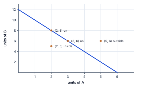
Units of B against units of A for a workshop that can make 12 B and no A, or 6 A and no B, with a constant trade-off of 2 B for each A. The frontier joins (0, 12) and (6, 0). The points (2, 8) and (3, 6) lie on it, using every resource. The point (2, 5) lies inside: feasible but leaving resources idle. The point (5, 6) lies outside: not feasible with these resources.

The figure draws the frontier from (0, 12) to (6, 0), with points on it, inside it and outside it.

The vertical intercept has A equal to zero and B at its maximum under the stated model. If a workshop can produce twelve B when it makes no A, that intercept is (0,12). The horizontal intercept has B equal to zero and A at its maximum. If that maximum is six, the horizontal intercept is (6,0). These two points answer different single-good allocation questions.

Zero is a meaningful quantity on both axes. It means none of that output is produced in the relevant plan; it does not mean that the axis is missing or that the producer has no resources. At an intercept, the resources may all be assigned to the other good. Omitting intercepts because they contain zero would remove two important feasible combinations from the graph.

Choose a scale large enough to contain every supplied point. If maximum A is six and maximum B twelve, both axes need not end at the same number. Equal physical lengths on the screen do not necessarily represent equal output quantities. This matters especially when later reading a slope: its economic units come from the axis scales, not from how steep a line happens to look in pixels.

Check an intercept against the resource account. With twelve hours, two hours per A, and one hour per B, the horizontal intercept is twelve divided by two, or six A. The vertical intercept is twelve divided by one, or twelve B. A plotted intercept of twelve A would assign all hours as if A used one hour each and would contradict the technology. The graph must agree with the underlying model, not merely fit inside its frame.

Another way: Connect points only when the model permits it

A table may list only a few combinations even when many intermediate allocations are feasible. Under divisible output and a constant resource trade-off, connecting the rows with a straight segment represents those additional combinations. For the frontier from (0,12) to (6,0), the intermediate point (3,6) is feasible because the shared resource account permits it. The line is justified by the production assumptions, not just by a desire for a smooth picture.

If production comes only in indivisible batches, the feasible set may consist of separate points rather than every point on a continuous line. Connecting points can still be a useful visual guide if explicitly described as such, but it should not claim that fractional output can actually be produced. A graph needs the same indivisibility conditions as the table it represents.

Likewise, a few collinear observed combinations do not by themselves prove that the entire true frontier is straight. A straight-line model assumes a constant opportunity cost over the relevant range. Resources with different suitability for tasks can produce changing costs and a curved or piecewise frontier. We can draw the supplied model precisely while acknowledging that additional evidence would be needed to establish its realism.

The plotting activities ask for the specified points. Their exact point keys assess whether coordinates have been translated correctly from the table. When teaching prose discusses a connecting frontier, it states the continuous constant-cost assumption explicitly. This distinction keeps a point-plotting exercise from silently claiming more about intermediate possibilities than its input supports.

Another way: Read movements and regions without changing the axes

Moving right on an A-horizontal graph means producing more A. Moving up means producing more B. Along a downward-sloping efficient frontier with fixed resources, moving right generally requires moving down: additional A is obtained by giving up some B. The picture expresses the production trade-off already present in the table. It does not imply that A has become more valuable or that B has become unwanted.

A movement from (2,8) to (4,4) increases A by two and reduces B by four. Keep the signs separate from the magnitudes. The change in B is negative four, while the amount of B forgone is positive four. Later, opportunity cost divides the quantity forgone by the quantity gained. In this lesson, identifying the direction and preserving the ordered pairs is the first task.

A point below the simple frontier may be feasible but use less than the model's productive capacity. A point above it requires more resources or a different technology than currently assumed. The next lessons examine those classifications in detail. For now, do not connect every observed output point and call the resulting path a frontier. Actual observations and an efficient possibility boundary are different objects.

Swapping the axes is allowed only if the labels and coordinates are swapped consistently. The same combination of two A and eight B would become (8,2) on a B-horizontal, A-vertical graph. It is not wrong to use that convention, but mixing it with an A-horizontal question is wrong. Our exercises keep the convention fixed to make the required reconstruction unambiguous.

Another way: Diagnose a misleading plot

The most common plotting mistake is a coordinate reversal. Check it by reading a point aloud in axis order. A point at horizontal two and vertical eight means two A and eight B under this lesson's convention. If the table row says eight A and two B, the point does not match, even though it uses the same two numbers. Correct numbers in the wrong positions are an incorrect production plan.

A second mistake is scale counting. If each horizontal grid step represents two A, the third step from zero represents six A, not three. Read the printed tick values rather than counting visible spaces as though every graph used the same scale. Digital point fields can accept numerical coordinates directly, but the displayed position still needs to be interpreted in the axis units.

A third mistake is combining both single-good maxima. The corner (maximum A, maximum B) usually lies beyond a two-good frontier because each maximum already uses the full resource stock separately. Check the resource demands of that corner. In the twelve-hour example, six A use twelve hours and twelve B use another twelve, so producing both would require twenty-four hours. Drawing the corner does not make it feasible.

Finish by comparing the plotted points with the table and assumptions. There should be one point for each requested row, with both intercepts included when supplied. Each pair should satisfy the same production rule. Any connecting interpretation should respect divisibility and constant-cost conditions. A clear graph makes those checks easier; it should not hide the model behind an appealing shape or an unlabeled line.

Another way: Resizing a picture does not change production

Stretching a graph vertically can make its frontier look steeper even though every numerical coordinate is unchanged. The production trade-off has not changed. Compare labeled quantities and their units rather than the angle a line makes on a particular screen. This matters when two otherwise identical graphs use different panel sizes or axis ranges: visual appearance alone cannot establish a different opportunity cost.

5. Plotting a workshop's afternoon choices

A fictional workshop has twelve productive hours. Product A needs two hours per unit and product B one. The frontier table lists (0,12), (2,8), (4,4), and (6,0), with A always first. The graph therefore labels its horizontal axis A units per afternoon and its vertical axis B units per afternoon. A horizontal maximum of six and vertical maximum of twelve accommodate every row.

The first point sits on the vertical axis at twelve, because it represents no A and twelve B. The last sits on the horizontal axis at six, because it represents six A and no B. The interior row (2,8) is two units across and eight up. Reversing it to (8,2) would put A beyond its single-good maximum and contradict the resource account.

Under a continuous constant-productivity model, the points lie on a straight segment. The intermediate combination (3,6) also uses twelve hours: three times two plus six times one. If outputs instead had to be made in the displayed batch quantities only, the line between plotted points would need a different interpretation. The graph's appearance cannot decide divisibility for us.

A viewer proposes marking (6,12) as the workshop's best possible combination because it contains both axis maxima. Checking its resource use gives twenty-four hours, twice the available capacity. The proposal confuses separate extremes with a simultaneous plan. The plotted frontier helps explain the error: every row describes one allocation of the same twelve hours, not permission to combine two complete uses of that stock.

6. Check the tempting inference

Do not reverse coordinates, combine both separate maxima, or infer units from screen distance alone. Plotting a few rows does not prove a continuous straight frontier; that interpretation needs the stated divisibility and constant-cost assumptions. Actual output observations need not lie on an efficient frontier.

7. Translate one interior row

8. Place the single-good extremes

9. Audit an entire frontier plot

10. Finish an axis-order check

11. Guided practice

A is horizontal, B vertical. One frontier table row gives A=3 and B=8. Enter the two coordinates in their labeled fields.

12. Guided practice

A is horizontal and B vertical. A supplied row has A=5, B=7. Complete the ordered-pair reasoning.

13. Guided practice

Plot all three supplied combinations, with A horizontal and B vertical: (0,12), (3,6), (6,0). These are rows of one constant-cost production model.

14. Practice

A is horizontal and B vertical. A single-good frontier row has A=10 and B=0. Enter its horizontal and vertical coordinates.

15. Practice

Plot the five rows of a production table, A horizontal and B vertical: (0,16), (2,12), (4,8), (6,4), (8,0). Plot points only; each row is a simultaneous pair.

16. Somewhere new

A fictional kitchen's fixed-resource table lists bread batches A and tray batches B: (0,10), (2,5), (4,0). Plot every pair with A horizontal and B vertical. These are production possibilities, not predicted orders.

17. Lesson test

Lesson test: one question per skill, one attempt each, no hints. Your answers are checked when you submit.

18. Test question

A fresh production table gives (A,B)=(0,18),(3,12),(6,6),(9,0). Plot every pair, keeping A horizontal and B vertical, including both intercepts.

19. What you can do now

Plot each simultaneous pair in axis order and check both extremes. State the assumptions needed to connect the points as a continuous straight frontier.

	Your result
Horizontal A coordinate
Vertical B coordinate