The production possibility table

Paper packet. Every task here also exists on screen, where it is checked automatically; answers written on paper are not assessed by Nydus. When you are back at a device, enter your answers there.

1. What you will learn

You will calculate the resources used by a chosen amount of one good, allocate the remainder efficiently to another, and verify the resulting production row against the shared constraint. Explain the constant-rate assumptions, distinguish possible from actual output, and avoid combining two single-good maxima as one simultaneous plan.

2. Starting point

Use the stated alternatives, quantities and units. Separate a model's assumptions from the conclusion derived from them.

3. Terms to use precisely

4. A production table describes possibilities, not wishes

A production possibility table lists combinations of two outputs that can be produced with specified resources, technology, and time. It makes a resource constraint visible in output units. A workshop with twelve available work-hours can devote some to product A and the remainder to product B. If each A requires two hours and each B one hour, the workshop cannot produce every desired quantity of both goods within twelve hours.

Start with the assumptions. The resource stock is fixed for the period. Each unit uses the stated number of hours, productivity is constant, and hours can be reassigned between the two activities. The exercise assumes no other bottleneck, no setup loss, and no production of additional goods. These are modeling choices, not observations that every workshop operates this simply. They allow us to derive a transparent table rather than guess its entries.

A row gives a pair of quantities produced together. Four A with four B uses twelve hours: four times two plus four times one. It does not mean that the workshop can separately produce four A and, using the whole budget again, twelve B. The two entries compete for the same resource stock. Read a row horizontally as one complete plan before comparing it with another row.

The table can describe frontier combinations using the resources efficiently under this model, or it can include other feasible combinations. A prompt should say which is intended. If it asks for the maximum B compatible with a stated A quantity, allocate the hours required for A and use the remaining productive hours for B. That procedure constructs a frontier row only because the simplified technology makes that remaining allocation efficient.

Term	What it means
Production possibility table	A list of output combinations feasible under stated resources and technology.
Resource requirement	The amount of a resource needed per unit of output.
Frontier combination	An efficient boundary combination with no feasible increase in one output without a reduction in another.
Constant productivity	An unchanged output-to-resource relationship over the allocations considered.
Resource account	The equation or inequality that prevents spending the same resource stock twice.

Another way: Use the resource equation before filling the table

For a fixed stock H of work-hours, a hours per A, and b hours per B, feasibility requires a times A plus b times B to be no greater than H. On the simple straight frontier, equality holds: all available productive hours are used efficiently. Writing this rule first gives every row the same basis and prevents the table from drifting into unrelated arithmetic.

Suppose H is twelve, a is two, and b is one. At A equal to zero, all twelve hours can produce B, so B is twelve. At A equal to two, A uses four hours, leaving eight for B. At A equal to four, A uses eight hours, leaving four for B. At A equal to six, A uses all twelve hours and B is zero. These paired rows come from one resource account.

The maximum output of a single good is found by assigning all relevant resources to it under the model. Maximum A is H divided by a, and maximum B is H divided by b. Do not multiply by hours per item when trying to find an item count. Twelve hours divided by two hours per A gives six A; twelve times two would produce units of hours squared per item rather than the required output.

For any proposed row, substitute its two outputs back into the resource rule. A row such as four A and five B would use thirteen hours in this example, exceeding capacity. A row such as four A and two B uses ten hours and is feasible but does not use the full productive capacity. This reverse check detects both impossible combinations and rows that have been mistakenly called frontier points.

Another way: Constant productivity creates a constant trade-off

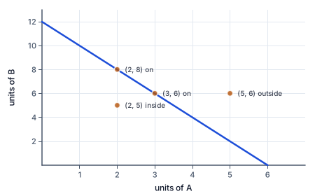
Units of B against units of A for a workshop that can make 12 B and no A, or 6 A and no B, with a constant trade-off of 2 B for each A. The frontier joins (0, 12) and (6, 0). The points (2, 8) and (3, 6) lie on it, using every resource. The point (2, 5) lies inside: feasible but leaving resources idle. The point (5, 6) lies outside: not feasible with these resources.

The figure plots a table like this one: with a constant trade-off, every row lies on one straight line.

In the model, moving two hours from B production to A production creates one additional A and gives up two B. The same reallocation has the same effect at every row because the per-unit resource requirements do not change. Constant opportunity cost produces a straight-line frontier when intermediate allocations are permitted. The next lesson turns that relationship into a graph.

Constant productivity does not mean that A and B require the same number of hours. Our example uses two hours per A and one per B. The relevant assumption is that the resource can be transferred without changing those rates across the allocations being compared. Saying that every worker is 'equally good at both goods' would be imprecise and could suggest an equality of outputs that the model does not require.

Real resources may be specialized. A worker or machine transferred early may be well suited to the new task, while a later transfer sacrifices more of the old output for the same gain. In that setting, opportunity costs can change and the frontier need not be straight. The simple table teaches how a constant-cost model works; it does not establish that every economy has constant costs.

The table's spacing is a presentation choice. We might list A quantities zero, two, four, and six, or include every whole A quantity. If divisible output and continuous allocation are assumed, additional intermediate combinations can lie between the displayed rows. If goods or resources are indivisible, not every point between rows is necessarily feasible. The model must state which interpretation applies before a line is drawn through the entries.

Another way: Capacity and actual production are separate

A production possibility table describes what could be produced under its conditions. Actual production can lie below that capacity because some resources are idle, coordination is poor, or another omitted constraint matters. A table derived from an idealized efficient technology is not a factual report that every resource is always employed in practice. Keep a model's feasible capacity separate from observations of output.

Even using all hours is not sufficient evidence of productive efficiency in a more complicated setting. Hours could be assigned to unsuitable tasks or wasted in avoidable delays. In this lesson's simple homogeneous-resource model, the stated constant rates and absence of other inefficiencies make full allocation a frontier condition. In a richer model, an efficient assignment must be established rather than assumed from a full timesheet.

A point inside the frontier may still be a deliberate choice under an objective that includes an omitted activity, such as rest, environmental protection, or maintenance. If those uses matter, the two-good model may be incomplete. The numerical classification 'inside' describes a relationship to the stated production possibilities; it does not by itself prove that the actual decision is socially undesirable. Later lessons distinguish productive possibilities from preferences over outcomes.

A change in the resource stock or technology requires a new table. If the workshop gains additional productive hours, the old boundary no longer describes all current possibilities. If one product requires fewer hours per unit, the output combinations also change. Do not alter a single row while pretending all assumptions remain the same. Explain which underlying parameter changed and derive the new rows consistently.

Another way: Check units, limits and the meaning of a row

A robust solution begins with the total resource unit and period, such as twelve workshop-hours this afternoon. It then states hours per A and hours per B. Multiplying output by hours per unit produces resource use; dividing remaining hours by hours per unit produces output. Writing those units beside the operations helps catch reversals before they become incorrect table entries.

Check the extreme rows. With zero A, B should reach its single-good maximum under the model. With maximum A, B should be zero. If a table claims positive B after A has already used every hour, it spends the resource stock twice. If increasing A also increases maximum B while capacity and technology are unchanged, the row construction likely violates the shared resource account.

Check one interior row separately. For a chosen A quantity, calculate its hours, subtract them from total capacity, and convert the remainder into B. Then add both goods' resource uses to verify the total. This is more reliable than continuing a visual number pattern without understanding why the pattern exists. A pattern can look regular even when its starting point or units are wrong.

Finally state the economic interpretation: this pair is the maximum compatible output of B for the chosen A under the given technology and resource stock. It is not a prediction that the workshop will choose the pair, nor proof that the pair is fairest or most valuable. The table supplies the opportunity set. A separate objective and any additional constraints are needed to select a plan from that set.

5. A workshop divides twelve productive hours

A fictional workshop has twelve productive machine-hours for one afternoon. A storage box requires two hours, while a simple tray requires one. Output uses only this machine time in the model, productivity is constant, and the machine can switch activities without losing time. The workshop wants to list the maximum trays compatible with several box quantities.

With no boxes, all twelve hours make twelve trays. Two boxes use four hours, leaving eight for eight trays. Four boxes use eight hours, leaving four for four trays. Six boxes use all twelve hours, leaving zero trays. The resulting pairs are (0,12), (2,8), (4,4), and (6,0), where the first number always means boxes and the second trays.

The manager proposes a fifth row: four boxes and five trays. Checking the resource account gives four times two plus five times one, or thirteen hours. The proposal is not feasible under the afternoon's twelve-hour capacity. Four boxes and two trays would use ten hours and would be feasible, but it would not be the maximum-tray row for four boxes under this simple model.

The table helps the manager identify a consistent menu of production plans. It does not choose the best mix, because the model has not supplied customer needs or the values of the outputs. It also does not establish that real switching time is always zero. If the workshop discovers a setup delay or another bottleneck, it should revise the assumptions and table together rather than treat the original arithmetic as evidence against the new fact.

6. Check the tempting inference

A table row is a simultaneous pair, not two separate maximum outputs. Constant productivity does not require equal hours per different good. A frontier is a capacity boundary under stated technology, not a prediction or a judgment of fairness. Full resource allocation implies efficiency here only because the simplified productive assumptions justify it.

7. An extreme row

8. An interior frontier row

9. Test a claimed production possibility

10. Finish a frontier row

11. Guided practice

A workshop has 24 hours; A needs 3 hours per unit, B needs 2. Set A=4. Under constant productivity and no other constraints, give A hours, remaining hours, and maximum B.

12. Guided practice

Capacity is 16 hours; A needs 4 hours and B needs 2 per unit. Set A=2 and complete the frontier row.

13. Guided practice

Capacity is 18 hours; A needs 3 and B needs 2 hours per unit. Set A=0. Give A resource use, remaining hours and maximum B.

14. Practice

Capacity is 30 hours; A needs 5 and B needs 3 per unit. Set A=6. Give A hours, remaining hours and maximum B.

15. Practice

Capacity is 28 hours; A needs 4 and B needs 2 per unit. Set A=3. Give A hours, remaining hours and maximum B; productivity is constant.

16. Somewhere new

A fictional community kitchen has 20 oven-hours. Loaf batch A needs 4 hours and tray batch B needs 2. It makes three A batches. With constant productivity, no setup loss and no other bottleneck, give A hours, remaining hours and maximum B batches.

17. Lesson test

Lesson test: one question per skill, one attempt each, no hints. Your answers are checked when you submit.

18. Test question

A new workshop has 36 productive hours. A uses 6 hours per unit and B uses 3. Set A=4. Give A hours, hours remaining and maximum compatible B under the constant-rate model.

19. What you can do now

Verify both intercepts and one interior row using the same resource equation. Explain which assumptions make the constructed rows frontier combinations.

	Your result
Hours used for A
Hours remaining for B
Maximum B units