Back to the on-screen lesson ·
Explain why nearby values may resemble each other.
Paper packet. Every task here also exists on screen, where it is checked automatically; answers written on paper are not assessed by Nydus. When you are back at a device, enter your answers there.
Define neighbors, measure adjacent similarity, and distinguish a spatial cluster from a tested explanation.
The previous lesson compared two variables within the same places. Here you compare one variable between connected places. Recall the mean, differences from a mean, and the rule that the product of two numbers with the same sign is positive. You will use these tools to inspect a spatial pattern without treating every observed location as an independent replicate.
| Term | What it means |
|---|---|
| Adjacency | A specified connection that makes two units neighbors. |
| Spatial autocorrelation | Similarity or dissimilarity of a variable across spatially related units. |
| Spatial weight | A number representing the strength of a neighbor connection. |
| Spatial outlier | A place unlike its defined neighbors. |
Spatial autocorrelation concerns a single variable measured at different locations. If neighboring places tend to have similar values, the pattern has positive spatial autocorrelation. If high values tend to neighbor low values, it has negative spatial autocorrelation. The word positive does not mean good, and negative does not mean harmful. These words describe a relationship between values and spatial connections. A cluster of high rents and a cluster of low rents can both contribute to positive autocorrelation.
Before describing clustering, define which places count as neighbors. Shared borders, distance thresholds, river connections and travel times represent different geographic processes. A bridge may connect two places that are far apart on a walking route but close on a road network. An island can have no land-border neighbor while remaining strongly linked by ferry. The choice of neighbors belongs in the explanation, because changing that choice can change the result. All grids and measurements in this lesson are fictional learning datasets.
Another way: table
| West-to-east position | Clustered canopy (%) | Alternating canopy (%) |
|---|---|---|
| 1 | 10 | 10 |
| 2 | 10 | 30 |
| 3 | 30 | 10 |
| 4 | 30 | 30 |
Imagine four blocks in a row. Under edge adjacency, block 1 connects to 2, block 2 to 3, and block 3 to 4. There are three unique undirected pairs. Do not count a block as its own neighbor. If you count both directions, the list has six directed connections, and every later sum must use that convention consistently. An unannounced switch between conventions doubles some quantities but not others.
For a two-dimensional grid, a shared-edge rule excludes diagonal contact, while a shared-corner rule includes it. Neither is universally correct. A fire spreading between contiguous buildings may motivate one rule; movement among park entrances may motivate travel-time weights. A statistical convenience is not a geographic justification.
Document the rule before examining which version gives a more dramatic result. Otherwise the analysis can become a search for a preferred conclusion. Include the treatment of isolated units. Quietly dropping an isolated settlement changes the population represented and can hide the most inaccessible places. If you add a nearest neighbor to every isolated unit, identify that exception and explain how it affects interpretation.
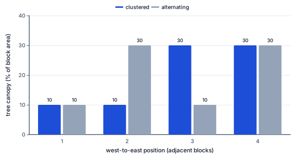
Use the sequence 10, 10, 30, 30 percent canopy. The absolute differences between adjacent blocks are 0, 20 and 0 percentage points. Their sum is 20 and their mean is about 6.67. Now rearrange the same values as 10, 30, 10, 30. Adjacent differences are 20, 20 and 20, giving a mean of 20. The alternating arrangement is rougher even though both arrangements contain exactly the same observations and have the same overall mean.
This mean adjacent difference is a transparent descriptive statistic. It is not Moran's I, a probability or a formal significance level. Small differences suggest similarity under the specified neighbor rule; their interpretation depends on the variable's scale. A difference of 10 in rainfall millimeters is not comparable with a difference of 10 in income currency units.
The comparison also shows why a histogram cannot recover geographic structure. Both sequences have two low values and two high values, so their histograms match. A map or an adjacency table is needed to reveal how those values are arranged. Preserve the location identifiers when exporting observations; sorting a spreadsheet by value destroys the original spatial sequence.
The mean of 10, 10, 30, 30 is 20. Deviations from the mean are minus 10, minus 10, plus 10 and plus 10. Multiplying deviations across each unique neighbor pair gives 100, minus 100 and 100. The positive total indicates that same-side-of-the-mean connections outweigh opposite-side connections in this simple unstandardized calculation. For the alternating sequence, every adjacent product is negative.
A standard autocorrelation statistic also normalizes for variation, sample size and the weights. You cannot label the raw product sum Moran's I or compare its magnitude across datasets with different measurement units. This course uses the products to explain the logic and keeps formal inferential spatial statistics outside its assessed scope.
Notice that equal values at two distant locations are not enough. Their contribution depends on whether the model connects them and with what weight. Similarly, a high block surrounded by low blocks can be a local outlier even if the region overall has positive autocorrelation. A regional summary must not erase a local exception that matters for field investigation.
Similarity can arise through diffusion, shared environmental conditions, common infrastructure or common policy. Adjacent farms may share soil properties; nearby rental markets may respond to the same station; neighboring disease reports may share a testing center. These are different mechanisms with different implications. A cluster identifies where to ask a question, not which mechanism is correct.
Spatial dependence matters when designing a sample. Ten sensors placed within the same small park may repeatedly measure the same local environment. They provide useful information about that park, but they do not necessarily offer ten independent pieces of evidence about the whole city. Spread sampling across relevant land uses and spatial zones, then record the remaining connections among sites.
Do not solve dependence by automatically discarding close observations. Fine spacing may be necessary to detect a sharp boundary or to estimate local exposure. Match the design to the question: mapping a road-edge gradient needs dense observations near the road, while estimating a citywide average needs coverage across the city. In both cases report the design instead of pretending locations were selected without spatial structure.
Check pair counting by drawing the graph of connections. A row of four units has three unique consecutive links; a closed ring of four adds the final-to-first link. With the clustered sequence, adding the closing link introduces another difference of 20. The mean difference becomes 40 divided by 4, or 10. The measured roughness changes because the topology changes, not because any canopy value changed.
Then test an alternative neighborhood motivated by the process. A one-block distance threshold may show strong local similarity, while a citywide all-pairs comparison includes many contrasting districts. Report the result at the scale tested. A map described as clustered without a neighbor definition is incomplete.
For claims about statistical significance, a suitable null model is also needed. Randomly relocating values can supply a reference distribution only if that relocation represents the null hypothesis sensibly. Coastlines, barriers and uneven sampling can make unrestricted shuffling inappropriate. Here the delivered calculations remain descriptive. They establish whether you can read connected values and compare arrangements; they do not certify an inferential spatial analysis or its assumptions.
At each position, compare the clustered and alternating arrangements. Both contain two values of 10 and two of 30, but the clustered sequence has only one contrasting neighbor link while the alternating sequence has three. Bar heights show canopy percent; position records west-to-east order, not time.
In a fictional district, three monitors within one courtyard record 18, 19 and 18 units, while a roadside monitor records 35. The courtyard mean of about 18.3 is a credible courtyard summary but a poor estimate of all district environments. Averaging the four sensors without considering placement gives the courtyard three times the influence of the road. A monitoring team should first define whether it wants population exposure, land-area conditions, or a comparison between traffic environments.
A redesigned survey could stratify locations into roadside, residential and park settings, then distribute observations within each. Repeated courtyard readings still help measure temporal variation. The improvement is not simply more equipment; it is a sampling design aligned with the geographic target. Privacy and access constraints must be documented rather than allowing convenient public sites to stand silently for every residence.
Four fictional fields along a drainage channel have crop-loss shares of 5, 5, 25 and 25 percent. The mean adjacent difference is 20 divided by 3 percentage points, revealing a sharp transition between the middle fields. A channel-borne process is one candidate, but a change in seed supplier at the same boundary is another. A useful follow-up samples upstream and downstream fields using the same seed, plus fields with different seeds away from the channel. That design separates hydrologic connection from supplier effects. Merely collecting more observations inside the high-loss patch would describe the patch more precisely without identifying its cause.
Positive spatial autocorrelation is a tendency toward similarity, not a rule that every adjacent pair matches. A transition zone can connect a high-value cluster to a low-value cluster. One unusual block does not disprove the entire regional tendency, and a regional tendency does not justify ignoring that block. Also distinguish spatial autocorrelation from a correlation between two variables: the former compares canopy with canopy at connected locations, whereas the latter might compare canopy with temperature in the same blocks.
Draw the four-unit row.
1—2—3—4
Only shared consecutive edges count.
List each unique connection.
1–2, 2–3, 3–4
Reverse directions are not new undirected pairs.
Count the listed pairs.
3 pairs
There is no link from 4 back to 1.
State the scope of the count.
A line topology with no isolated nodes.
A ring would require a different list.
Read the clustered values.
10, 10, 30, 30
Positions remain west to east.
Take absolute adjacent differences.
0, 20, 0
Absolute values measure roughness without direction.
Average the differences.
20 / 3 = 6.67 approximately
There are three unique links.
Read the alternating arrangement.
10, 30, 10, 30
The values and mean have not changed.
Compare its mean difference.
60 / 3 = 20
Arrangement changes local similarity.
Find the overall mean.
(10 + 10 + 30 + 30) / 4 = 20
The four units have equal weight.
Write deviations in spatial order.
-10, -10, 10, 10
Centering makes high and low relative to the mean.
Multiply across the three links.
100, -100, 100
Same-sign products are positive.
Add the unstandardized products.
100 - 100 + 100 = 100
Positive links outweigh the transition link.
Identify the exception.
The middle pair crosses low to high.
A cluster can contain a boundary.
Avoid an unsupported statistic.
This sum is not Moran's I or a p-value.
Normalization and a reference model are absent.
List neighboring absolute differences.
0, 20, 0
Keep the spatial order.
Sum the differences.
20
Two edges have no contrast.
Divide by the number of edges.
A row has canopy values 13, 13, 40, 40. Which statement distinguishes spatial autocorrelation from ordinary two-variable association?
Complete the calculation. A fictional row has 2 neighbor links, each with an absolute canopy difference of 32 percentage points. What is the total adjacent difference?
Multiply each link difference by the number of links.
r
Sum one difference per link; equal differences allow multiplication.
Check that every unique link contributes once.
Check the units and the stated comparison.
Double counting changes the total.
Keep this descriptive sum separate from a significance claim.
Keep the result within the supplied observations.
Define the neighbor graph before interpreting similarity; a cluster alone does not identify its cause.
Order a reproducible canopy roughness calculation.
Number the steps in order (write the number in the box):
A river-linked crop-loss cluster is being investigated. Select evidence that distinguishes water transport from a shared seed supplier.
This task has no paper form; do it on a device.
Match the observed arrangement to its interpretation.
| Positive local similarity under the stated links | Negative local similarity under the stated links | A candidate local spatial outlier | |
|---|---|---|---|
| Low beside low and high beside high | |||
| High beside low throughout | |||
| One high block among low neighbors |
A fictional row has 4 neighbor links, each with an absolute canopy difference of 35 percentage points. What is the total adjacent difference?
Answer: summed percentage points
A four-block line has values 0, 0, 20, 20. Enter the total squared-free absolute difference if each link is counted in both directions. Then do the same for 0, 20, 0, 20.
| summed percentage points | |
|---|---|
| Clustered directed total | |
| Alternating directed total |
A researcher samples 4 sensors inside one park and one beside a highway, then calls the park sensors independent evidence for the whole city. Which revision best addresses the spatial design?
Lesson test: one question per skill, one attempt each, no hints. Your answers are checked when you submit.
Four invented adjacent plots form a line; only consecutive plots are neighbors. Arrangement A is 20, 20, 31, 31 percent canopy. Arrangement B is 20, 31, 20, 31. Sum absolute differences across the three links in each arrangement and calculate B minus A. This is an arrangement diagnostic, not Moran's I.
| summed percentage points | |
|---|---|
| A total adjacent difference | |
| B total adjacent difference | |
| B minus A |
Explain how the same observations can look clustered under one neighbor definition and mixed under another.
17. For a line with values 5, 5, 25, 25, complete the mean adjacent difference., step 3
20 / 3 = 6.67 approximately
Count links rather than locations.