Fieldwork limits · printable packet

Field readings are few: the median resists unusual values that pull the mean, the interquartile range sets fences for outliers, and one day may not represent a place.

Paper packet. Every task here also exists on screen, where it is checked automatically; answers written on paper are not assessed by Nydus. When you are back at a device, enter your answers there.

1. What you will learn

By the end of this lesson you will be able to summarize field readings, flag outliers with the interquartile range, and say what a small sample can and cannot show.

2. What you already have

You can design a sample. This lesson takes the readings a sample gives and asks what they can and cannot show: which summaries to trust, how to spot an unusual value, and why a few readings from one day may not describe a place.

3. Words for this lesson

4. What a handful of readings can show

Term	What it means
Mean	The total of the readings divided by how many there are.
Median	The middle reading when they are put in order.
Quartiles	The values a quarter and three quarters of the way through the ordered readings.
Interquartile range	The upper quartile less the lower: the spread of the middle half.
Outlier	A reading more than one and a half interquartile ranges beyond a quartile.
Representative	Describing the whole place and time, not only where and when it was measured.

Another way: picture

Picture ten friends comparing their allowance, and then a billionaire walks in. The average allowance in the room jumps to millions, but the middle person's allowance has not changed. The mean tells you about the billionaire; the median tells you about the room.

Another way: steps

Put the readings in order.
Find the median and the quartiles.
Compute the interquartile range and the fences.
Flag readings beyond the fences, and check them.
Report the mean and median, and say when and where the data came from.

5. Sensitivity to resolution and boundaries

A fieldwork conclusion should survive reasonable changes in representation, or explicitly report where it fails. Resolution changes the support of a raster value: a coarse cell can combine several land-cover patches. A boundary change alters which land or people enter a summary and its denominator. Resampling does not collect new evidence. Compare dates, class definitions, masks and population denominators before interpreting a difference as real change.

Use a small controlled comparison. In a fictional tree-cover survey, site P has 70 percent and Q 60 percent with fine cells and original boundaries. With coarse cells and the same boundaries they have 65 and 62 percent, retaining the ranking. With fine cells and revised boundaries they have 55 and 64 percent, reversing it. A fourth run with coarse cells and revised boundaries tests their combined effect. These supplied results suggest boundary sensitivity in this example. They do not show that trees disappeared between dates. Check the underlying observations before proposing that mechanism.

6. Reporting what survived the check

State the original claim precisely: a ranking, a threshold decision or a magnitude. A ranking may survive while its margin shrinks enough to make the decision uncertain. Conversely, a regional total may stay stable while local hotspots disappear. Keep a table of controlled runs and note which factors changed. If both boundaries and cell size change in a single comparison, you can diagnose lack of robustness but cannot isolate the cause. Rerun one factor at a time, and include combinations if the effects may interact. A transparent report can conclude that more detailed observations are needed. It should not delete the unfavorable run or describe a method-driven change as an observed environmental trend.

7. Seeing the spread

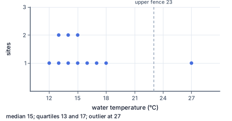
The dot plot shows water temperature at eleven sites along a stream. Ten sites lie between 12 and 18 degrees, around a median of 15, with quartiles of 13 and 17. One site reads 27 degrees, alone to the right, beyond the upper fence of 23.

Before deciding what that dot means, go back to the site: a thermometer left in the sun, a mistyped number, or warm water flowing out of a factory pipe just upstream would each explain it, and only the last is a finding.

8. Mean and median

The mean of the eleven stream readings is $174 \div 11 \approx 15.8$ degrees; the median is 15. The single warm site pulls the mean up by almost a degree, while the median stays with the typical sites.

Data with a long tail on one side, such as rainfall, incomes or home prices, is better described by the median, which is why the typical home price is reported as a median.

9. Quartiles and the interquartile range

Ordered readings are split into quarters. The lower quartile, $Q_1$, is the median of the lower half; the upper quartile, $Q_3$, the median of the upper half. For the stream, $Q_1 = 13$ and $Q_3 = 17$, so the interquartile range is $4$.

Unlike the range, 15 degrees for the stream, the interquartile range ignores the extremes, so one odd reading cannot inflate it.

10. The outlier rule

A common rule flags any reading more than one and a half interquartile ranges beyond a quartile. For the stream, $1.5 \times 4 = 6$, so the fences are $17 + 6 = 23$ and $13 - 6 = 7$. The reading of 27 is beyond the upper fence.

The rule is a flag, not a verdict. It says which readings deserve a second look.

11. Keep, fix or explain

A flagged reading has three fates. If it was a recording error, such as 72 typed for 27, fix it and note the fix. If the instrument failed, drop it and say why. If it is real, keep it: it may be the most important thing the fieldwork found.

Deleting inconvenient readings without a reason is not cleaning data; it is changing the answer.

12. When and where

A stream measured on a hot August afternoon will read warmer than the same stream at dawn in April. Readings from one day describe that day, not the season.

Good fieldwork records the date, time, weather and exact location of every reading, and repeats measurements at other times when the question is about a whole year.

13. Small samples

Five rain gauges in a county can easily miss a thunderstorm that soaked one neighborhood. A small sample can be fair and still unlucky.

The fewer the readings, the more cautious the conclusion: report the numbers, the sample size and what the sample could have missed.

14. The method, step by step, and how to check it

Checking an answer. The median lies between the quartiles. The upper fence is above the upper quartile and the lower fence below the lower. When the data has a long upper tail, the mean exceeds the median.

15. Why each step is allowed

Using the median as the center is allowed because it depends on order, not on how far the extremes reach. Measuring spread with quartiles is allowed for the same reason.

The factor of one and a half is a convention, chosen by the statistician John Tukey so that, for bell-shaped data, very few ordinary readings are flagged.

16. Volunteers and quality

Much American environmental data comes from volunteers: stream monitors, bird counters and backyard rain gauges. Programs train them, give them the same instruments and check their readings against each other and against official stations.

Flagging outliers is part of that checking. A gauge that reads twice its neighbors every storm may be under a gutter.

17. Common slips

The most common slip is deleting outliers without checking them. Another is reporting the mean of skewed data as if it were typical.

A third is adding one interquartile range instead of one and a half for the fence. A fourth is drawing conclusions about a season from a single day.

18. Limits as data

Every fieldwork result is shaped by its sample, its instruments and its timing. The last lesson of the course turns to people: how the choices made in collecting and mapping data can help or harm the communities it describes.

19. In the world: a rain gauge in every backyard

In July 1997 a storm dropped more than ten inches of rain on parts of Fort Collins, Colorado, flooding a creek and killing five people. Official gauges had missed how concentrated the rain was. The next year, the Colorado Climate Center started the Community Collaborative Rain, Hail and Snow Network, CoCoRaHS, which asks volunteers to read identical gauges each morning.

The network has spread to every state, with thousands of observers. Their readings fill the gaps between official stations and feed flood forecasts and drought maps.

Quality control is built in: a reading far from its neighbors is flagged and checked with the observer. Sometimes it is a typo; sometimes it is the one backyard under the heaviest cell of a storm, exactly the kind of reading the network was created to catch.

20. In the world: why home prices are medians

When the National Association of Realtors reports what homes cost in the United States, it reports the median price of existing homes sold, not the mean. The Census Bureau does the same for household income.

The reason is the shape of the data. A few very expensive sales or very high incomes pull the mean far above what a typical buyer pays or a typical household earns. On a street where four homes sell for 300 thousand dollars and one for 1.3 million, the mean is 500 thousand, a price nobody on the street paid.

The mean still has a use, for totals such as the value of all sales or a county's tax base, which is why careful reports give both and say which is which.

21. An outlier is a question, not a mistake

It is tempting to treat any reading far from the rest as an error and delete it, so the data looks tidy. But an outlier may be a real event: a warm outflow, a local downpour, a polluted well. Deleting it can erase the very thing the fieldwork was meant to find.

The rule only flags readings. Each flagged one is checked, and then fixed with a reason, dropped with a reason, or kept and explained.

22. Mean and median of rain gauges

23. Fences for a stream

24. Home prices

25. Your turn: readings have quartiles $30$ and $40$. Find the fences.

26. Guided practice

A set of stream readings has a lower quartile of $30$ and an upper quartile of $50$. Above what value is a reading flagged as an outlier?

27. Guided practice

Complete the worked solution: soil moisture readings on a field trip have a lower quartile of $12$ and an upper quartile of $18$ percent. Find the interquartile range, the upper fence and the lower fence.

28. Guided practice

29. Practice

Five rain gauges in a county recorded $4$, $6$, $7$, $9$ and $24$ millimeters in one storm. Fill in the mean, the median and the range.

30. Practice

A student's readings so far total $72$. After one more reading $x$ there are $4$ readings. Write the new mean as a function of $x$.

31. Practice

A survey of commute times has a lower quartile of $20$ minutes and an upper quartile of $30$ minutes. Below what time is a commute flagged as an outlier?

32. Somewhere new

Suppose five homes sold on a street this year: four for $200$ thousand dollars each and one for $700$ thousand. By how many thousand dollars does the mean sale price exceed the median?

33. Somewhere new

Mark sentences establishing the observed sensitivity, attribution limit and controlled recheck. A fictional study ranks 4 parks using one dated image. With 10 m cells and original boundaries, A has 60% mapped habitat and B 50%. With 30 m cells and revised boundaries, A has 45% and B 55%.

34. Lesson test

Lesson test: one question per skill, one attempt each, no hints. Your answers are checked when you submit.

35. Test question

A student's readings so far total $90$. After one more reading $x$ there are $6$ readings. Write the new mean as a function of $x$.

36. What you can do now

You can reason about fieldwork limits. Explain why a flagged outlier should be checked rather than deleted.

Working for the steps left to you

	value
mean (mm)
median (mm)
range (mm)

25. Your turn: readings have quartiles $30$ and $40$. Find the fences., step 3

One and a half ranges below.