Back to the on-screen lesson ·
Interpret scales, denominators, grouped data and multiple-answer questions across common displays.
Paper packet. Every task here also exists on screen, where it is checked automatically; answers written on paper are not assessed by Nydus. When you are back at a device, enter your answers there.
Extract the quantities needed from a display, calculate a supported result and select all and only the statements established by the data.
Review percentages, ratios, weighted means and descriptive statistics. A total count and a rate answer different questions. A percent increase uses the initial value as the denominator. A frequency table's mean weights each value by its count. A boxplot summarizes ordered positions without normally revealing every observation. These relationships remain the same whether the data are shown as a table or graph; only the extraction step changes.
| Term | What it means |
|---|---|
| Legend | The key connecting symbols, colors or lines to represented groups. |
| Frequency | The number of observations in a value or interval category. |
| Scale | The relationship between a displayed position or length and its numerical value. |
| Association | A pattern relating two variables, which alone does not establish causation. |
Data interpretation begins before arithmetic. Read the title, labels, units, legend and notes to determine what the numbers represent. A table entry of twenty can mean twenty people, twenty thousand dollars or twenty percent of a specified group. A graph's apparent visual contrast can depend on its scale. The task is to extract the relevant evidence and perform the requested comparison, not to calculate every possible summary in the display.
GRE quantitative data sets can support single-selection, multiple-selection and numeric-entry questions. In a select-all item, judge each option independently and choose all and only the supported statements. The number of correct choices may vary. Our multiple-selection activities use exact-set grading, so selecting a plausible unsupported extra claim does not preserve credit for the true statements you also selected.
Another way: steps
Read the display metadata; identify the requested quantities; normalize units and denominators; compute or compare; reject claims beyond the evidence.
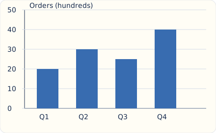
These bars show orders in hundreds. Q1 represents two thousand orders and Q4 four thousand. Their ratio is two to one, while the difference is two thousand orders. A chart with a truncated vertical axis can make a modest numerical difference look dramatic, so use the labeled values rather than comparing visible bar lengths blindly. Categorical bars can be separated because their horizontal positions identify categories, not continuous intervals. A color difference has meaning only if the legend assigns one.
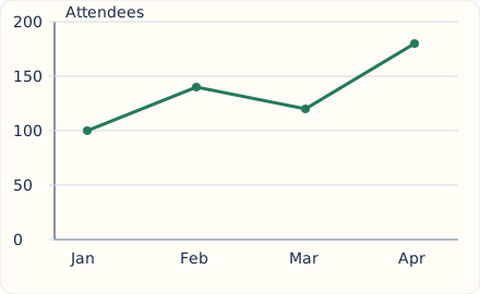
The largest month-to-month increase is from March to April, sixty attendees. January to February rises forty, while February to March falls twenty. Connecting monthly observations makes the sequence visible but does not establish a measurement on every intervening day or a linear process between endpoints. Extending the last segment into a future month is a prediction requiring a model, not a value observed in the graph. If horizontal intervals differ, compare rates of change using the elapsed time as well as vertical change.
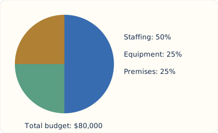
The staffing sector is half of an eighty-thousand-dollar budget, or forty thousand dollars. Each quarter sector represents twenty thousand. A sector's angle is its share times 360 degrees. When comparing two circle charts, equal sector percentages need not represent equal amounts because the totals may differ. A ten-percent share of a million exceeds a twenty-percent share of one hundred thousand. Identify each chart's whole before comparing parts, and check that categories are intended to be mutually exclusive when summing shares.
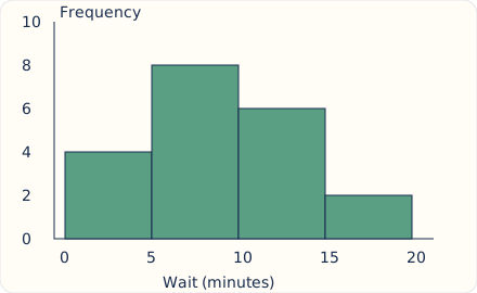
These equal-width bins contain twenty observations in total, with eight in the interval from five inclusive to ten exclusive minutes. The interval notation decides where a boundary value belongs. Grouping generally hides the exact values inside each bin, so multiplying midpoints by frequencies gives an estimate of the mean, not necessarily the exact mean. With unequal-width bins, a density histogram can use area rather than height to represent frequency; read the vertical label before treating every height as a count. Adjacent bins represent intervals, unlike separate categorical bars.
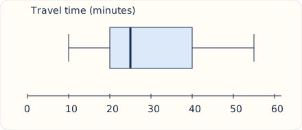
The box spans Q1 twenty to Q3 forty, giving an interquartile range of twenty minutes. The median is twenty-five, and the stated whiskers mark a range from ten to fifty-five. The four quartile regions can have different numeric widths even though each represents roughly a quarter of ordered positions under the display's convention. A longer region does not mean more observations in it. Do not infer the exact mean, sample size or individual observations from this five-number summary alone.
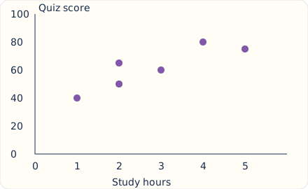
Each point pairs hours with a score for one observation. The overall pattern is positive, but the points do not lie on one exact line. Two observations share two study hours while having different scores, showing that the plotted relationship is not a deterministic function from hours to score. The plot does not establish that additional study caused the score differences; other factors or selection effects may contribute. A trend can support a bounded association statement without supporting a causal or universal claim.
Do not infer that a question must have two correct options because the previous one did. For each proposed statement, identify the cells, points or summaries that would establish it. Compute separately where needed. A statement about a percentage needs its own denominator; a causal statement needs more than a before-and-after change; an exact mean cannot usually be recovered from grouped intervals. Mark a claim false or unsupported for a specific reason. Only after evaluating every option should you compare your selected set with the task's directions.
A dashboard comparing branches may highlight total errors because those counts are easy to display. To compare error rates, divide by the workload for each branch. Then inspect whether the branches handled comparable cases before drawing a causal conclusion about staff performance. Correct normalization repairs a numerical comparison, but it does not automatically establish why the rates differ.
A second dashboard might present monthly totals using a vertical axis that begins near the smallest value. Read the tick labels and calculate the difference directly. You can acknowledge a real increase while rejecting the impression that one value is several times another.
In review, classify errors into extraction, scale, denominator, calculation or overclaim. Extraction errors need practice locating the correct series or cell. Denominator errors need a written ratio. Overclaims need attention to what the display cannot establish. This targeted record is more useful than repeatedly calculating an already familiar average. Use fresh displays for a later check, and preserve your initial select-all response before reading the explanations.
A taller bar may be exaggerated by a truncated scale. A greater count need not mean a greater rate. A histogram bin does not place all observations at its midpoint. Boxplots do not ordinarily reveal an exact mean. A connected line does not establish continuous measurement or future values. A scatterplot association is not a causal demonstration.
Read the scale label.
Revenue is listed in thousands: year one 72, year two 90.
The question requests the dollar increase.
Subtract values in table units.
90 - 72 = 18.
The difference is eighteen thousand-dollar units.
Convert to requested units.
18 times 1000 = 18,000 dollars.
The label controls the scale of the response.
Distinguish a percent question.
The percent increase would be 18/72 times 100 = 25 percent.
That is a different target despite using the same two cells.
Read each numerator and denominator.
Branch P has 6 errors in 60 cases; branch Q has 9 errors in 150 cases.
The question compares error rates.
Compute the first rate.
6/60 = 10 percent.
Use P's own case count.
Compute the second rate.
9/150 = 6 percent.
Use Q's own larger workload.
Compare rates and counts separately.
Q has more errors but a lower error rate.
Both statements can be true because the denominators differ.
Limit the interpretation.
The table alone does not identify the cause of the rate difference.
Case difficulty or other conditions could differ between branches.
Read interval boundaries and frequencies.
Bins [0,5), [5,10), [10,15) contain 3, 8 and 5 observations.
The intervals include left endpoints and exclude right endpoints.
Recover the total count.
3 + 8 + 5 = 16.
All displayed observations are included once.
Locate the median positions.
The eighth and ninth observations are in the middle bin.
Its cumulative positions run from four through eleven.
Evaluate a percentage claim.
Five sixteenths are at least ten and below fifteen.
The last bin supplies the numerator.
Reject an exact-mean claim.
The actual positions inside each interval are unknown.
Different within-bin values can keep the histogram unchanged while altering the mean.
Reject an endpoint-as-observation claim.
The graph does not establish that any observation equals fifteen.
Fifteen is excluded from the last bin rather than reported as a measured maximum.
Read both totals and shares.
A category is 20 percent of 500 in one chart and 25 percent of 320 in another.
The percentage alone does not decide the amount comparison.
Compute each represented amount.
0.20 times 500; 0.25 times 320.
Compare the products using the same units.
State the supported comparison.
A table records shipments: North 120, South 180, West 300. What percentage of the total came from South? Select one answer.
A company's revenue, in thousands of dollars, was 80 in year A and 100 in year B. What was the increase in dollars? Select one answer.
Quarterly orders are Q1: 40, Q2: 60, Q3: 50, Q4: 90. From Q3 to Q4, what is the percent increase? Select one answer.
A frequency table shows score 2: 3 students; score 3: 4 students; score 5: 1 student. What is the mean score? Select one answer.
A circle chart assigns 45 percent of a 240,000-dollar budget to staffing. How many dollars go to staffing? Select one answer.
A boxplot reports Q1=12, median=18 and Q3=27. What is the interquartile range? Select one answer.
Monthly visits were January 100, February 150, March 120 and April 180. Select all supported statements.
A histogram has equal-width bins: [0,10) contains 5 observations; [10,20) contains 9; [20,30) contains 6. Select all statements established by these grouped data.
A scatterplot consists of points (1,3), (2,5), (3,4), (4,8), (5,9), where x is study hours and y is a quiz score. Select all supported statements.
A table reports product A: 40 units at 15 dollars each; product B: 30 units at 20 dollars each; product C: 20 units at 25 dollars each. Select all supported statements.
A service dashboard shows branch A processed 80 applications with 8 errors and branch B processed 200 with 12 errors. Which statement correctly compares their error rates? Select one answer.
Lesson test: one question per skill, one attempt each, no hints. Your answers are checked when you submit.
A boxplot is explicitly defined with whiskers at the minimum and maximum. Its five values are 4, 10, 16, 22 and 34, in order. Select all supported statements.
Tomorrow, compare a count with a rate, read a boxplot's legend and explain why grouped histogram data may not determine an exact mean. Then answer a fresh select-all question by evaluating each option independently.
17. Complete a circle-chart comparison, step 3
The amounts are 100 and 80; the smaller percentage represents the larger amount.
Different wholes can reverse an ordering based only on shares.