Back to the on-screen lesson ·
Use probability weights, expected values, symmetry and standard-deviation units.
Paper packet. Every task here also exists on screen, where it is checked automatically; answers written on paper are not assessed by Nydus. When you are back at a device, enter your answers there.
Compute bounded conclusions from a stated probability distribution without treating expected values or normal approximations as guarantees.
Review weighted means, complement probabilities and the fact that probabilities lie between zero and one. For a finite exhaustive list of mutually exclusive outcomes, their probabilities must sum to one. A frequency distribution counts observations; a probability distribution assigns probabilities. Dividing frequencies by their total creates relative frequencies, which can be used as a model when the question specifies that interpretation. A graph alone should be read with its axis labels to determine whether it shows counts, proportions or density.
| Term | What it means |
|---|---|
| Random variable | A numerical quantity determined by an outcome of a chance process. |
| Expected value | The probability-weighted mean of the possible values. |
| Standardized value | The distance from the mean divided by the standard deviation. |
| Normal distribution | A continuous symmetric bell-shaped model specified by a mean and a positive standard deviation. |
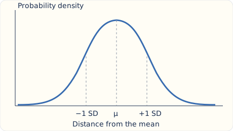
A random variable assigns a numerical value to each outcome of a chance process. Its probability distribution describes which values can occur and how much probability each receives. A discrete distribution may be displayed in a short table. A continuous model such as a normal distribution describes probabilities over intervals using area under a curve. The height of the curve at a point is not the probability of that exact value. In a continuous normal model, a single exact value has probability zero, while an interval can have positive probability because it spans an area under the curve.
A summary of a distribution is not a prediction that one particular trial must equal that summary. Expected value is a probability-weighted average. It can lie between possible outcomes and may never occur on a single trial. Standard deviation describes spread about that average, while the shape controls how probability is allocated around it. Keep these roles separate when interpreting a model or comparing two groups.
Another way: steps
Identify possible values and probability weights; check the distribution; choose a weighted average or interval argument; interpret the result within the stated model.
Each listed probability must be nonnegative and no greater than one. If the rows contain all possible values, the probabilities must add to one. A missing probability can be found by subtracting the known sum from one. If that subtraction gives a negative result, the proposed model is invalid rather than an unusual distribution. Rows for different values of one discrete random variable are mutually exclusive, so probabilities of a set of values can be added directly. Include zero when a question asks for a nonnegative value; positive and nonnegative define different events.
For values x1, x2 and so on with corresponding probabilities p1, p2 and so on, expected value is the sum of each x times its p. If a variable is zero with probability three quarters and eight with probability one quarter, its expected value is two even though two is impossible on a single trial. The result describes a long-run average in repeated realizations of the model, not a guaranteed single outcome. A value with the largest probability is a mode, which need not equal the expected value.
If a random variable X has expected value m, then aX + b has expected value am + b. A fixed fee shifts every possible cost and therefore shifts the mean by the same amount. Scaling each outcome scales the mean accordingly. This does not require independence because only one variable and constants are involved. For a sum of random variables, expectations also add without an independence assumption, although statements about the variance of a sum require more care. Do not extend a correct mean rule automatically to every other summary.
A normal distribution is symmetric about its mean, where mean, median and mode coincide. Half its probability lies below the mean and half above. Intervals equally far to either side have equal probability. If the mean is forty and the standard deviation five, the interval thirty-five to forty mirrors forty to forty-five. Symmetry alone does not tell you the probability in either interval; for that you need a supplied area, an accepted approximation or a table. Distinguish what follows from symmetry from what requires numerical information.
Subtract the mean from an observation and divide by the positive standard deviation. The resulting z value states how many standard deviations above or below the mean the observation lies. An observation below the mean has a negative z value. If one test has a much larger raw-score scale than another, raw differences from the mean cannot be compared directly. Standardized values place those differences in their own spread units. This comparison does not by itself show that the distributions are normal or that the same z value has the same percentile in differently shaped distributions.
For a normal model, a common approximation places about sixty-eight percent within one standard deviation, ninety-five percent within two and 99.7 percent within three. These rounded figures are not exact identities. If ninety-five percent lies centrally, the remaining five percent is split equally between the two tails, giving about 2.5 percent above the upper two-standard-deviation boundary. Read whether a question asks for a central interval, one tail or both tails. In our numerical practice, the required approximation is supplied so the expected response is unambiguous.
Knowing a mean and standard deviation does not establish a normal distribution. A skewed or bimodal distribution can share those summaries with a normal one. Applying the sixty-eight-percent rule without a normal assumption is therefore unjustified. A histogram can suggest a shape, but a small sample's appearance does not prove a population model. For bounded test questions, use the distributional assumption explicitly supplied. For a reading interpretation, preserve uncertainty and avoid turning a model-based approximation into a claim about every individual observation.
If expected delivery time is four days and every shipment receives an additional fixed two-day processing period, expected total time becomes six days. This follows because every possible delivery outcome shifts by the same two days. It does not imply every customer waits exactly six days or that six is the most frequent observed duration.
If instead processing time varies, its expected value can still be added to expected delivery time, but conclusions about the total spread require information about their joint behavior. A delay in one stage may be associated with a delay in another. Do not assume independence merely to obtain a convenient formula.
For practice, separate three statements in your review notes: the model's assumption, the calculation under that assumption and the interpretation supported by the result. This separation is especially useful when a normal approximation is supplied. You can calculate the requested tail accurately while still recognizing that the approximation is conditional on the stated normal model and does not guarantee an individual outcome.
An expected value need not occur in one trial and need not be the most likely outcome. A normal curve's height is not a point probability. A negative standardized value is valid, but standard deviation is nonnegative. Symmetry supplies equal areas, not every numerical area. A mean and standard deviation do not establish normality.
Check the probability total.
Values 0, 2 and 6 have probabilities 0.5, 0.25 and 0.25.
The probabilities are nonnegative and sum to one.
Weight each possible value.
0(0.5)=0; 2(0.25)=0.5; 6(0.25)=1.5.
The weights describe how much each value contributes to the mean.
Add the weighted contributions.
Expected value = 2.
The weighted total is zero plus one half plus one and one half.
Interpret the result correctly.
Two is the mean, while zero is the most probable single value.
Expected value and mode answer different questions.
Read location and spread.
A measurement has mean 120 and standard deviation 16.
Find the standardized position of 96.
Compute the signed displacement.
96 - 120 = -24.
The observation lies below the mean.
Express the displacement in spread units.
-24/16 = -1.5.
Each standard-deviation unit is sixteen raw units.
State the position.
The observation is 1.5 standard deviations below the mean.
The negative sign describes direction, not negative spread.
Respect the model's limits.
A percentile cannot be recovered from these summaries alone.
The distribution's shape or additional probability information is needed.
Read the supplied model.
A normal variable has mean 60 and standard deviation 4.
Use the approximation that ninety-five percent lies within two standard deviations.
Locate the central interval.
60 - 8 = 52; 60 + 8 = 68.
Two standard deviations span eight units in either direction.
Find the probability outside the interval.
100 percent minus 95 percent equals 5 percent.
This combines both tails.
Use symmetry to separate the tails.
Each tail contains approximately 2.5 percent.
The normal model makes the tails equal.
Answer the requested upper-tail question.
Approximately 2.5 percent of values exceed 68.
Five percent would incorrectly include the lower tail as well.
Preserve approximation language.
The result uses the stated rounded ninety-five-percent rule.
It is not an exact probability derived solely from the mean and standard deviation.
Read all mutually exclusive outcomes.
A variable has only three possible values with probabilities 0.1, p and 0.6.
Their probabilities must sum to one.
Solve for the missing weight.
p = 1 - 0.1 - 0.6.
Check the resulting value lies between zero and one.
Verify the completed distribution.
A random variable takes values 0, 1 and 2 with probabilities 0.2, 0.5 and 0.3. What is its expected value?
Answer:
A measurement has mean 50 and standard deviation 8. A value of 66 is how many standard deviations above the mean?
Answer:
A random variable takes values 2, 4 and 10 with probabilities 0.25, 0.5 and 0.25. What is its expected value?
Answer:
A distribution assigns probabilities 0.15, 0.35 and p to its only three outcomes. What is p?
Answer:
A random variable takes values -2, 0 and 3 with probabilities 0.2, 0.5 and 0.3. What is the probability it is nonnegative?
Answer:
A normal distribution has mean 100 and standard deviation 15. What value lies 2 standard deviations below the mean?
Answer:
For a normal distribution, use the approximation that 68 percent of values lie within one standard deviation of the mean. Approximately what percent lie between the mean and one standard deviation above it?
Answer:
For a normal distribution, use the approximation that 95 percent of values lie within two standard deviations of the mean. Approximately what percent lie above the mean plus two standard deviations?
Answer:
A variable X has expected value 7. What is the expected value of 3X - 4?
Answer:
A measurement has mean 24 and standard deviation 6. What is the standardized value of an observation of 15?
Answer:
A delivery time has expected value 4 days. A service adds a fixed 2-day processing period to every delivery. What is the expected total time in days?
Answer:
Lesson test: one question per skill, one attempt each, no hints. Your answers are checked when you submit.
A normal distribution has mean 72 and standard deviation 9. What value is one standard deviation above its mean?
Answer:
Tomorrow, explain why an expected value need not be an attainable outcome. Then locate an observation in standard-deviation units and separate exact normal symmetry from an approximate central-area rule.
17. Complete a probability-table check, step 3
p = 0.3; the three probabilities total one.
The table now assigns a valid weight to every possible value.