Back to the on-screen lesson ·
Convex and concave functions, $E[f(X)]$ against $f(E[X])$, and the inequality that proves Gibbs' inequality and every entropy bound after it.
Paper packet. Every task here also exists on screen, where it is checked automatically; answers written on paper are not assessed by Nydus. When you are back at a device, enter your answers there.
By the end of this lesson you will be able to state Jensen's inequality for convex and concave functions and say which way it points for each common function, compute the gap it predicts in small cases exactly, identify when it is an equality, assemble the proof of Gibbs' inequality from it, and recognise it at work outside the course, where the average of a logarithm and the logarithm of an average come apart.
Expected values, the second derivative as the test for a curve bending up or down, and the entropy bound $H \le \log_2 n$ quoted in the last lesson as resting on Gibbs' inequality. This lesson supplies the one inequality Gibbs, and nearly everything after it, rests on.
A function is convex when every chord — the segment joining two points of its graph — lies on or above the graph, and concave when every chord lies on or below. Jensen's inequality compares $E[f(X)]$ with $f(E[X])$, and the Jensen gap is their difference; it is zero in the equality case, when $X$ is constant.
A function $f$ is convex when every chord lies on or above its graph, $f(\lambda x + (1 - \lambda) y) \le \lambda f(x) + (1 - \lambda) f(y)$, and concave when the reverse holds; $x^2$ and $2^x$ are convex, $\log x$ and $\sqrt{x}$ are concave. Jensen's inequality extends the chord to any distribution: for convex $f$, $$E[f(X)] \ge f(E[X]),$$ and for concave $f$, $E[f(X)] \le f(E[X])$, with equality for strictly convex or concave $f$ exactly when $X$ is constant. The gap for $f(x) = x^2$ is the variance. Information theory uses Jensen with $f = \log$: it proves Gibbs' inequality $D(p \| q) \ge 0$, the bound $H(X) \le \log_2 n$, the concavity of entropy in the distribution, and the convexity of relative entropy. The log-sum inequality, $\sum a_i \log \frac{a_i}{b_i} \ge (\sum a_i) \log \frac{\sum a_i}{\sum b_i}$, is Jensen in disguise and does the same work in proofs about channels.
Another way: picture
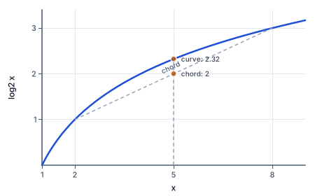
The graph of $\log x$ with two points marked and the chord between them: the chord's midpoint, $E[\log X]$, sits below the curve at $E[X]$. For $x^2$ the picture flips, and the vertical gap between chord and curve is the variance.
Another way: steps
A function is convex when the chord between any two points of its graph lies on or above the graph, concave when it lies on or below. The quickest test is the second derivative: $f'' \ge 0$ means convex, $f'' \le 0$ means concave, and a strict sign means strictly convex or concave. The graph below shows the concave $\log_2 x$ with the chord from $(2, 1)$ to $(8, 3)$: above $x = 5$, the average of the two logs is $2$ while the log of the average is $2.32$.
| $f(x)$ | $f''(x)$ | shape | Jensen says |
|---|---|---|---|
| $x^2$ | $2$ | convex | $E[X^2] \ge (E[X])^2$ |
| $2^x$ | $(\ln 2)^2\, 2^x$ | convex | $E[2^X] \ge 2^{E[X]}$ |
| $1/x$ ($x > 0$) | $2/x^3$ | convex | $E[1/X] \ge 1/E[X]$ |
| $x \log_2 x$ | $1/(x \ln 2)$ | convex | used for the convexity of $D$ |
| $\log_2 x$ | $-1/(x^2 \ln 2)$ | concave | $E[\log_2 X] \le \log_2 E[X]$ |
| $\sqrt{x}$ | $-\tfrac{1}{4} x^{-3/2}$ | concave | $E[\sqrt{X}] \le \sqrt{E[X]}$ |
| $h(p)$ | $-1/(p(1 - p) \ln 2)$ | concave | mixing coins raises entropy |
For two points the inequality is the definition of convexity: $X = x_1$ with probability $\lambda$ and $x_2$ with probability $1 - \lambda$ has $E[X] = \lambda x_1 + (1 - \lambda) x_2$ and $E[f(X)] = \lambda f(x_1) + (1 - \lambda) f(x_2)$, the height of the chord. For $n$ points, peel off the last one: write $E[X]$ as a two-point mixture of $x_n$ and the conditional mean of the others, apply the two-point case, and use induction on the rest. For continuous $X$ the same argument works with a supporting line at $E[X]$: a convex $f$ lies above its tangent, $f(x) \ge f(\mu) + f'(\mu)(x - \mu)$, and taking expectations kills the linear term.
For $f(x) = x^2$ the gap has a name: $E[X^2] - (E[X])^2 = \operatorname{Var}(X)$. For a two-point $X$ taking $a$ or $b$ with probability $\tfrac{1}{2}$ each it is $\tfrac{(a - b)^2}{4}$, the square of half the distance between the points:
| $X = a$ or $b$, equally likely | $E[X]$ | $E[X^2]$ | gap $E[X^2] - (E[X])^2$ |
|---|---|---|---|
| general $a, b$ | $\tfrac{a + b}{2}$ | $\tfrac{a^2 + b^2}{2}$ | $\tfrac{(a - b)^2}{4}$ |
| $1, 3$ | $2$ | $5$ | $1$ |
| $2, 8$ | $5$ | $34$ | $9$ |
| $4, 4$ | $4$ | $16$ | $0$ |
For the logarithm and $X = 2^i$ or $2^j$ equally likely, $E[\log_2 X] = \tfrac{i + j}{2}$ exactly, while $\log_2 E[X] = \log_2 \tfrac{2^i + 2^j}{2}$ is larger unless $i = j$: with $i = 1, j = 3$ that is $2$ against $\log_2 5 = 2.322$.
Common mistakes
The first error is reversing the direction for concave functions; picture the chord, below the curve for $\log$ and above it for $x^2$, and the direction follows. The second is claiming equality when $E[X] = 0$, or when $X$ is symmetric about its mean; for a strictly convex $f$ equality needs $X$ constant, and no special mean will do. The third is mixing the two sides: computing $f$ of each value and then squaring the average, or averaging and then forgetting to apply $f$. Keep $E[f(X)]$ and $f(E[X])$ apart on paper, and the gap between them is the whole content of the inequality.
$X = 2$ or $8$, each with probability $\tfrac{1}{2}$. $E[X] = 5$, $\log_2 5 \approx 2.322$.
$f$ of the mean.
$E[\log_2 X] = \tfrac{1}{2}(1 + 3) = 2 \le 2.322$: concave, so the mean of the logs is smaller.
The mean of the logs.
$-D(p \| q) = \sum p \log_2 \dfrac{q}{p} = E_p\left[\log_2 \dfrac{q(X)}{p(X)}\right]$.
Write the divergence as an expectation of a log.
Jensen (concave $\log$): $\le \log_2 E_p\left[\dfrac{q}{p}\right] = \log_2 \sum q = 0$, so $D(p \| q) \ge 0$.
Equality only when $q/p$ is constant, i.e. $p = q$.
$E[X] = 5$, so $f(E[X]) = 25$.
$E[X^2] = \tfrac{9 + 49}{2} = 29$.
Square first, then average.
Gap $= 29 - 25 = 4 = \tfrac{(7 - 3)^2}{4}$, the variance of $X$.
$\log_2 1 = 0$ and $\log_2 16 = 4$, so $E[\log_2 X] = \tfrac{0 + 4}{2} = 2$.
$E[X] = 8.5$ and $\log_2 8.5 = 3.087$.
$\log_2 8.5 = 3 + \log_2 1.0625 \approx 3 + 0.087$.
$2 \le 3.087$: the concave logarithm turns the average of the logs into less than the log of the average, by more than a bit here because the points are far apart.
$E[\sqrt{X}] = \tfrac{1}{2}(1 + 3) = 2$ and $\sqrt{E[X]} = \sqrt{5} \approx 2.236$.
$2 \le 2.236$, as Jensen requires for the concave square root.
For a random variable $X$ on the positive reals, match each function $f$ to the relation Jensen's inequality gives between $E[f(X)]$ and $f(E[X])$.
| $E[f(X)] \ge f(E[X])$ | $E[f(X)] \le f(E[X])$ | $E[f(X)] = f(E[X])$ for every $X$ | |
|---|---|---|---|
| $f(x) = x^2$ | |||
| $f(x) = \log_2 x$ | |||
| $f(x) = \sqrt{x}$ | |||
| $f(x) = 2^x$ | |||
| $f(x) = 9x + 1$ |
$X$ equals $2$ or $8$ with probability $\tfrac{1}{2}$ each, and $f(x) = x^2$. Fill in $E[X]$, $f(E[X])$, $E[f(X)]$ and the Jensen gap $E[f(X)] - f(E[X])$.
| Value | |
|---|---|
| $E[X]$ | |
| $f(E[X])$ | |
| $E[f(X)]$ | |
| Gap |
$X$ equals $2$ or $32$ with probability $\tfrac{1}{2}$ each. Compute $E[\log_2 X]$ and compare it with $\log_2 E[X]$; enter $E[\log_2 X]$.
Answer:
Build the proof of Gibbs' inequality, $D(p \| q) \ge 0$ with equality only for $p = q$, from Jensen's inequality.
This task has no paper form; do it on a device.
Each round, a gambler's wealth is multiplied by $2$ or by $\tfrac{1}{2}$, each with probability $\tfrac{1}{2}$. Let $W$ be the factor for one round. Fill in $E[\log_2 W]$, which governs the typical long-run growth, and $E[W]$, the expected factor.
| Value | |
|---|---|
| $E[\log_2 W]$ | |
| $E[W]$ |
Lesson test: one question per skill, one attempt each, no hints. Your answers are checked when you submit.
For a strictly convex $f$, when does Jensen's inequality $E[f(X)] \ge f(E[X])$ hold with equality?
You can decide the direction of Jensen's inequality, compute its gap, and derive Gibbs' inequality from it. Say in your own words why the equality case for a strictly convex function needs a constant variable and nothing less. Next: entropy of several variables at once, and the chain rule.
13. Your turn: $X = 1$ or $9$ equally likely; compare $E[\sqrt{X}]$ and $\sqrt{E[X]}$, step 2