Back to the on-screen lesson ·
The bounds $0 \le H \le \log_2 n$, the distributions that attain each end, and why a function of $X$ never carries more entropy than $X$.
Paper packet. Every task here also exists on screen, where it is checked automatically; answers written on paper are not assessed by Nydus. When you are back at a device, enter your answers there.
By the end of this lesson you will be able to prove that entropy lies between $0$ and $\log_2$ of the number of outcomes, say exactly which distributions attain each end, explain why a function of a random variable never has more entropy than the variable itself, sort statements about entropy into the ones that always hold and the ones that do not, and use these bounds to check any entropy you compute.
Entropy as average surprise, exact for dyadic distributions, and the binary entropy function with its peak at the fair coin. This lesson asks how large and how small an entropy can be at all, and which distributions sit at the ends.
The support of a distribution is the set of outcomes with positive probability, and $n$ counts them. The uniform distribution gives each of them $1/n$. A function of $X$, $Y = f(X)$, merges outcomes of $X$ that share a value of $f$. Gibbs' inequality, $D(p \| q) \ge 0$, is quoted here and proved two lessons on.
Every term $p \log_2 (1/p)$ is nonnegative, so $H(X) \ge 0$, and $H(X) = 0$ exactly when one outcome has probability $1$. At the other end, $H(X) \le \log_2 |\mathcal{X}|$ with equality only for the uniform distribution: the proof compares $p$ with the uniform $u$ through Gibbs' inequality $D(p \| u) \ge 0$, which unfolds to $\log_2 n - H(X) \ge 0$. Two further facts follow the same pattern. A function of $X$ has no more entropy than $X$: $H(f(X)) \le H(X)$, with equality when $f$ is injective on the support, because merging outcomes can only make the variable more predictable. And relabelling outcomes changes nothing, since $H$ depends only on the multiset of probabilities. These bounds are the sanity checks for every computation in the course: a result outside $[0, \log_2 n]$ is wrong.
Another way: picture
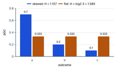
A bar chart of a distribution being flattened step by step toward equal bars: every step that moves probability from a taller bar to a shorter one raises the entropy, until the bars are level at the maximum $\log_2 n$.
Another way: steps
Let $p$ be any distribution on $n$ outcomes and $u(x) = 1/n$ the uniform one. Gibbs' inequality (proved in lesson 4 from Jensen) says $D(p \| u) \ge 0$. Expand the divergence: $$D(p \| u) = \sum_x p(x) \log_2 \frac{p(x)}{1/n} = \sum_x p(x) \log_2 p(x) + \sum_x p(x) \log_2 n = -H(X) + \log_2 n.$$ So $\log_2 n - H(X) \ge 0$, and the gap between the maximum and the actual entropy is exactly $D(p \| u)$. Equality in Gibbs needs $p = u$, so only the uniform distribution reaches $\log_2 n$. The lower bound is easier: every term $p \log_2 (1/p)$ is $\ge 0$, and the sum is $0$ only when each term is, which forces every $p(x)$ to be $0$ or $1$: a single certain outcome.
| Distribution on $3$ outcomes | $H$ | $\log_2 3$ | gap $= D(p \| u)$ |
|---|---|---|---|
| $(1, 0, 0)$ | $0$ | $1.585$ | $1.585$ |
| $(0.7, 0.2, 0.1)$ | $1.157$ | $1.585$ | $0.428$ |
| $(0.5, 0.3, 0.2)$ | $1.485$ | $1.585$ | $0.100$ |
| $(0.4, 0.4, 0.2)$ | $1.522$ | $1.585$ | $0.063$ |
| $(\tfrac{1}{3}, \tfrac{1}{3}, \tfrac{1}{3})$ | $1.585$ | $1.585$ | $0$ |
Read the table downwards: as the bars flatten, the entropy climbs toward $\log_2 3$ and the gap shrinks to $0$. The gap is never negative.
Why can $Y = f(X)$ never have more entropy than $X$? Use the chain rule (lesson 3) on the pair $(X, Y)$ twice. Since $Y$ is determined by $X$, $H(Y \mid X) = 0$ and $H(X, Y) = H(X) + H(Y \mid X) = H(X)$. But also $H(X, Y) = H(Y) + H(X \mid Y) \ge H(Y)$. Hence $H(Y) \le H(X)$, with equality exactly when $H(X \mid Y) = 0$, that is when $X$ can be recovered from $Y$: $f$ is injective on the outcomes that actually occur. The lost amount $H(X \mid Y) = H(X) - H(f(X))$ is how much of $X$ the function threw away.
| $X$ uniform on | $Y = X \bmod m$ | values of $Y$ | $H(Y)$ | $H(X \mid Y) = H(X) - H(Y)$ |
|---|---|---|---|---|
| $\{1, \ldots, 16\}$ | $m = 4$ | $4$ | $2$ | $4 - 2 = 2$ |
| $\{1, \ldots, 16\}$ | $m = 2$ | $2$ | $1$ | $4 - 1 = 3$ |
| $\{1, \ldots, 64\}$ | $m = 8$ | $8$ | $3$ | $6 - 3 = 3$ |
| $\{1, \ldots, 2^{j + m}\}$ | $m = 2^j$ | $2^j$ | $j$ | $m$ |
The pattern in the last row is the one the practice uses: when $X$ is uniform on $2^{j + m}$ values, $X \bmod 2^j$ is uniform on $2^j$ residues (each residue is hit by exactly $2^m$ values), so $H(Y) = j$ bits and the function discarded $m$ bits. By contrast $Y = X^2$ on positive values is injective, so $H(X^2) = H(X)$: squaring loses nothing.
Common mistakes
The commonest slip is writing $n$ instead of $\log_2 n$ for the maximum: ten values allow $3.322$ bits, not $10$. The second is believing a spread of large numbers has more entropy than a spread of small ones; only the probabilities matter, and relabelling changes nothing. The third is answering $H(Y) = H(X)$ for $Y = X \bmod m$: the residue forgets the quotient, and $H(Y)$ is $\log_2 m$ only when $X$ is uniform on a multiple of $m$ values. And the equality cases are sharp: $H = \log_2 n$ needs the uniform distribution, not merely a spread-out one.
Let $u$ be uniform on the $n$ outcomes. Gibbs: $D(p \| u) = \sum p \log_2 \dfrac{p}{1/n} \ge 0$.
Relative entropy against the uniform.
Expand: $\sum p \log_2 p + \sum p \log_2 n = -H(X) + \log_2 n \ge 0$.
$\sum p = 1$ pulls $\log_2 n$ out.
So $H(X) \le \log_2 n$, with equality only when $p = u$.
Gibbs is tight only at equality of the distributions.
$X$ uniform on $\{1, \ldots, 8\}$, $H(X) = 3$; $Y = X \bmod 2$ takes two values, each from four $X$ values, so $Y$ is a fair bit.
Compute the distribution of $Y$.
$H(Y) = 1 \le 3 = H(X)$: merging outcomes lost two bits.
$H(f(X)) \le H(X)$.
Six outcomes allow at most $\log_2 6 = 2.585$ bits.
$\log_2 6 = \log_2 2 + \log_2 3 = 1 + 1.585$.
The distribution $(0.5, 0.1, 0.1, 0.1, 0.1, 0.1)$ has $H = 0.5 \cdot 1 + 5 \cdot 0.1 \cdot 3.322 = 0.5 + 1.661 = 2.161$ bits.
$2.161 \le 2.585$ as it must be; the gap $0.424$ is $D(p \| u)$.
$H(X) = \log_2 32 = 5$ bits.
Each residue $0, 1, 2, 3$ is hit by exactly $8$ of the $32$ values, so $Y$ is uniform on $4$ values and $H(Y) = 2$ bits.
Uniform in, uniform out, because $4$ divides $32$.
The function discarded $H(X \mid Y) = 5 - 2 = 3$ bits: the quotient, which takes $8$ equally likely values.
The maximum is $\log_2 5 \approx 2.322$ bits.
$2.5 > 2.322$: no such distribution exists.
A random variable takes $4$ values. Give the set of values its entropy $H$, in bits, can possibly take, as an interval.
This task has no paper form; do it on a device.
Build the proof that a random variable with $n$ values has $H(X) \le \log_2 n$, with equality only for the uniform distribution.
This task has no paper form; do it on a device.
$X$ is uniform on $\{1, 2, \ldots, 32\}$ and $Y = X \bmod 2$. Fill in how many values $Y$ takes, and the entropies of $Y$ and of $X$, in bits.
| Value | |
|---|---|
| Number of values of $Y$ | |
| $H(Y)$ in bits | |
| $H(X)$ in bits |
$X$ takes $6$ values. Select every statement that is true for every distribution of $X$.
This task has no paper form; do it on a device.
A hash table has $16$ buckets and a key is drawn uniformly from $128$ possible keys; the hash sends exactly $8$ keys to each bucket. What is the entropy, in bits, of the bucket the key lands in?
Answer:
Lesson test: one question per skill, one attempt each, no hints. Your answers are checked when you submit.
Sort each distribution by where its entropy sits: at zero, at the maximum $\log_2 n$ for its number of values, or strictly between.
| $H = 0$ | $H = \log_2 n$, the maximum | strictly between $0$ and $\log_2 n$ | |
|---|---|---|---|
| $(1, 0, 0)$ | |||
| $(\tfrac{1}{3}, \tfrac{1}{3}, \tfrac{1}{3})$ | |||
| $(\tfrac{1}{2}, \tfrac{1}{4}, \tfrac{1}{4})$ | |||
| $(\tfrac{1}{4}, \tfrac{1}{4}, \tfrac{1}{4}, \tfrac{1}{4})$ | |||
| $(0.9, 0.1)$ |
You can bound entropy, name the extreme distributions, and say how much a function of a variable forgets. Say in your own words why the uniform distribution is the only one at the top of the range, and what a certain outcome does to the bottom. Next: Jensen's inequality, the convexity tool behind every entropy inequality.
13. Your turn: can a distribution on $5$ outcomes have entropy $2.5$ bits?, step 2