Back to the on-screen lesson ·
$\nabla \cdot \vec{E} = \rho/\varepsilon_0$ and $\nabla \times \vec{E} = 0$: divergence and curl in Cartesian and spherical coordinates, charge densities from fields, and the divergence theorem as a check.
Paper packet. Every task here also exists on screen, where it is checked automatically; answers written on paper are not assessed by Nydus. When you are back at a device, enter your answers there.
By the end of this lesson you will be able to compute the divergence and curl of electric fields, find charge densities from fields, and test whether a field can be electrostatic.
You know Gauss's law in integral form, $\oint\vec{E} \cdot d\vec{a} = Q_{\text{enc}}/\varepsilon_0$, from Physics C, and from multivariable calculus the gradient, divergence and curl and the divergence and Stokes theorems. You can compute fields of distributions by integrating Coulomb's law. This lesson turns the integral laws into statements about every point in space.
| Term | What it means |
|---|---|
| Del operator | $\nabla = \hat{x}\,\partial_x + \hat{y}\,\partial_y + \hat{z}\,\partial_z$, a vector of derivatives. |
| Divergence | $\nabla \cdot \vec{E}$, the net outflow of a field per unit volume at a point. |
| Curl | $\nabla \times \vec{E}$, the circulation of a field per unit area at a point. |
| Flux | $\oint\vec{E} \cdot d\vec{a}$, the field's flow through a closed surface. |
| Divergence theorem | $\int_V\nabla \cdot \vec{F}\,d\tau = \oint_S\vec{F} \cdot d\vec{a}$. |
| Stokes's theorem | $\int_S(\nabla \times \vec{F}) \cdot d\vec{a} = \oint_C\vec{F} \cdot d\vec{l}$. |
| Conservative field | A field with zero curl, which is the gradient of a potential. |
Gauss's law says the flux through any closed surface equals the enclosed charge over $\varepsilon_0$. Apply the divergence theorem to the left side, write the charge as $\int\rho\,d\tau$, and since the volume is arbitrary the integrands must match:
$$\nabla \cdot \vec{E} = \frac{\rho}{\varepsilon_0}.$$
The divergence measures how much field flows out of a small volume, per unit volume. Where there is positive charge, field lines begin; where there is none, every line that enters leaves again. In Cartesian coordinates $\nabla \cdot \vec{E} = \partial_xE_x + \partial_yE_y + \partial_zE_z$; for a radial field in spherical coordinates it is $\frac{1}{r^2}\frac{d}{dr}(r^2E_r)$.
The Coulomb field of a point charge also has zero curl, and by superposition so does every electrostatic field:
$$\nabla \times \vec{E} = 0.$$
By Stokes's theorem, the line integral of $\vec{E}$ around any closed loop vanishes, so the work done moving a charge between two points is independent of path, and $\vec{E}$ is the gradient of a potential, $\vec{E} = -\nabla V$. These two differential equations, together with boundary conditions, determine the electrostatic field completely; the rest of electrostatics is solving them.
Another way: picture
Picture the field as the velocity of a steady fluid. Divergence asks whether a tiny box has more fluid leaving than entering: a source inside, like a spring on a pond. Curl asks whether a tiny paddle wheel placed in the flow would spin. Electrostatic fields are like water spreading from springs and draining into sinks, never swirling in eddies: sources and sinks are charges, and there are no whirlpools.
Another way: steps
Checks. The Coulomb field $kq\hat{r}/r^2$ must give zero divergence everywhere except the origin, where the charge is. A uniform field must give zero. The total charge found by integrating $\rho$ over a volume must match $\varepsilon_0$ times the flux out of its surface. And any field claimed to be electrostatic must pass the curl test in all three components.
Consider a radial field $E_r(r)$ and a thin spherical shell between $r$ and $r + dr$. The flux out through the outer surface is $E_r(r + dr)\,4\pi(r + dr)^2$ and in through the inner surface $E_r(r)\,4\pi r^2$. The difference is $4\pi\,d(r^2E_r)$, and dividing by the shell's volume $4\pi r^2\,dr$ gives $\frac{1}{r^2}\frac{d}{dr}(r^2E_r)$.
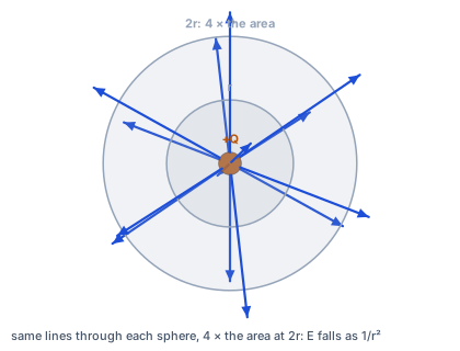
The $r^2$ appears because spherical surfaces grow with radius. A field that falls as $1/r^2$ keeps $r^2E_r$ constant: the same flux passes through every sphere, so no charge lies between them. That is why the Coulomb field has zero divergence away from the point charge, even though it is not constant. In cylindrical coordinates the surfaces grow as $s$, so a $1/s$ field, like a line charge's, has zero divergence away from the line.
In the figure, field lines begin on the charge and nowhere else. Around it, in empty space, every line that enters a small volume also leaves it, which is zero divergence.
For $\vec{E} = kq\hat{r}/r^2$, the formula gives $\nabla \cdot \vec{E} = 0$ for every $r > 0$, yet the flux through any sphere around the origin is $q/\varepsilon_0$. All the divergence is concentrated at a single point. Mathematically,
$$\nabla \cdot \frac{\hat{r}}{r^2} = 4\pi\,\delta^3(\vec{r}),$$
where the three-dimensional delta function is zero everywhere except the origin and integrates to one. A point charge's density is $\rho = q\,\delta^3(\vec{r})$, and Gauss's law in differential form holds even there.
Delta functions let point charges, line charges and surface charges be treated with the same equations as smooth densities. Surface charges produce jumps in the field rather than infinite divergence, and those jumps give the boundary conditions of the lessons on conductors and dielectrics.
A curl-free field can be written as the gradient of a scalar function. That replaces three unknown components with one unknown potential, and it turns Gauss's law into a single second-order equation, Poisson's equation, $\nabla^2V = -\rho/\varepsilon_0$. It also makes energy accounting simple: the work to move a charge depends only on the endpoints, so potential energy is well defined.
Zero curl is special to electrostatics. When magnetic fields change in time, Faraday's law gives $\nabla \times \vec{E} = -\partial\vec{B}/\partial t$, and the electric field can circulate; that circulating field drives the current in every electric generator and transformer. The curl test is therefore also a way to tell whether a field comes from charges alone or from changing magnetism too.
Gauss's law in differential form lets you find where charge is by measuring the field, without seeing the charge. Atmospheric physicists do exactly this. On fair-weather days the air carries a downward field of about $100$ to $150$ V/m at the ground, weakening with height. The weakening means a net positive space charge in the air, about $\rho = \varepsilon_0\,dE_z/dz$, of order a few femtocoulombs per cubic meter near the ground: a few more positive ions than negative ones in each cubic centimeter.
The same idea underlies many instruments. Field mills on towers at Kennedy Space Center measure the atmospheric field before launches, because strong fields and the charge they reveal signal a risk of triggered lightning. In semiconductor devices, measuring or modeling how the field changes across a junction gives the charge of the ionized dopants that create it.
The integral form of Gauss's law is powerful but needs symmetry to solve for $\vec{E}$. The differential form works at every point with no symmetry at all. Combined with zero curl, it gives Poisson's and Laplace's equations, which can be solved analytically for many geometries and numerically for any. Every electrostatic simulation, from the design of a capacitor to the modeling of a protein's electrostatic surface, solves these differential equations on a grid.
The differential form also generalizes. Maxwell's four equations are all written with divergence and curl, and in that form they reveal their structure: sources of divergence (charges), sources of curl (currents and changing fields), and the absence of magnetic charge. Learning to compute and interpret divergence and curl now is learning the language of the rest of the course.
Real problems rarely come in Cartesian form, and the formulas for divergence and curl change with coordinates because the unit vectors do. In cylindrical coordinates $(s, \phi, z)$, the divergence is $\frac{1}{s}\partial_s(sE_s) + \frac{1}{s}\partial_\phi E_\phi + \partial_zE_z$. In spherical coordinates $(r, \theta, \phi)$, it is $\frac{1}{r^2}\partial_r(r^2E_r) + \frac{1}{r\sin\theta}\partial_\theta(\sin\theta\,E_\theta) + \frac{1}{r\sin\theta}\partial_\phi E_\phi$.
These look forbidding but reduce to one term for fields with symmetry. Keep a reference table at hand, as every physicist does; the skill is recognizing which term matters and applying it correctly, not memorizing all of them.
Earth's surface carries a net negative charge of about half a million coulombs, maintained by thunderstorms worldwide, and the upper atmosphere a matching positive charge. In fair weather this produces a downward field of about $100$ to $150$ V/m at the ground: between your head and your feet there is a potential difference of about $200$ volts, harmless because air conducts so poorly.
The field weakens with height, falling to a few volts per meter by $10$ km, and by Gauss's law that weakening reveals positive space charge in the lower atmosphere. Measurements from towers, balloons and aircraft, used in the global atmospheric electric circuit studies that began at the Carnegie Institution in Washington in the early twentieth century, map that charge. The Carnegie curve — the daily cycle of the fair-weather field, peaking at 19:00 Greenwich time when thunderstorms over the Americas are most active — was one of the first discoveries made this way.
Engineers designing high-voltage equipment, microchips and particle detectors do not integrate Coulomb's law by hand. They discretize space into a grid or mesh and solve $\nabla \cdot \vec{E} = \rho/\varepsilon_0$ and $\nabla \times \vec{E} = 0$, usually as Poisson's equation for the potential. Finite-element programs used across American industry replace each derivative with differences between neighboring grid points and solve millions of coupled equations.
A standard test of such software is exactly this lesson's check: compute the flux out of a closed surface numerically and compare it with the charge inside. If the divergence theorem fails in the simulation, the mesh is too coarse or the boundary conditions are wrong. The same differential equations, in their full time-dependent form, run inside the simulations used to design antennas, microwave ovens and the radio-frequency cavities of particle accelerators.
A strong field does not mean charge is present, and a weak one does not mean it is absent. The Coulomb field is enormous near a point charge yet has zero divergence everywhere except at the charge itself: the field weakens exactly fast enough to keep the flux through every sphere the same. A uniform field, however strong, has zero divergence. Charge shows up only where the field's flux changes from place to place.
A second error is to apply the Cartesian formula to a field written in spherical coordinates, differentiating $E_r$ with respect to $r$ and stopping. That gives the Coulomb field a nonzero divergence and a uniform ball the wrong density. The geometric factors, $r^2$ in spherical and $s$ in cylindrical coordinates, are not optional.
Take the field $\vec{E} = (2x, 3y, 4z)$ V/m² times position. Differentiate $E_x$.
$\partial_xE_x = 2$
Each component with respect to its own coordinate.
Differentiate the $y$ component.
$\partial_yE_y = 3$
$E_y = 3y$.
Differentiate the $z$ component.
$\partial_zE_z = 4$
$E_z = 4z$.
Add the derivatives.
$\nabla \cdot \vec{E} = 9\ \text{V/m}^2$
The same at every point.
Find the charge density.
$\rho = 8.85 \times 10^{-12} \times 9 = 7.97 \times 10^{-11}\ \text{C/m}^3$
A uniform density of about $80$ pC/m³.
Write the field inside a uniform ball of radius $R$ and charge $Q$.
$\vec{E} = \dfrac{kQr}{R^3}\hat{r}, \quad r < R$
From Gauss's law in integral form.
Multiply by $r^2$.
$r^2E_r = \dfrac{kQr^3}{R^3}$
Prepare for the spherical divergence.
Differentiate with respect to $r$.
$\dfrac{d}{dr}(r^2E_r) = \dfrac{3kQr^2}{R^3}$
The power rule.
Divide by $r^2$.
$\nabla \cdot \vec{E} = \dfrac{3kQ}{R^3}$
Constant inside the ball.
Find the charge density.
$\rho = \varepsilon_0 \cdot \dfrac{3Q}{4\pi\varepsilon_0R^3} = \dfrac{Q}{\tfrac{4}{3}\pi R^3}$
Exactly the charge divided by the volume.
Check outside the ball.
$r > R: \ r^2E_r = kQ \quad\Rightarrow\quad \nabla \cdot \vec{E} = 0$
No charge outside, as it should be.
Take $\vec{E} = cr^2\hat{r}$ inside a region. Compute the divergence.
$\nabla \cdot \vec{E} = \dfrac{1}{r^2}\dfrac{d}{dr}(cr^4) = 4cr$
Spherical divergence of a radial field.
Write the charge density.
$\rho = 4\varepsilon_0cr$
Increasing outward.
Integrate the density out to radius $R$.
$Q = \displaystyle\int_0^R4\varepsilon_0cr \cdot 4\pi r^2\,dr = 16\pi\varepsilon_0c\dfrac{R^4}{4} = 4\pi\varepsilon_0cR^4$
Shells of volume $4\pi r^2\,dr$.
Compute the flux through the sphere of radius $R$.
$\oint\vec{E} \cdot d\vec{a} = cR^2 \times 4\pi R^2 = 4\pi cR^4$
The field is radial and uniform on the sphere.
Multiply the flux by $\varepsilon_0$.
$\varepsilon_0\oint\vec{E} \cdot d\vec{a} = 4\pi\varepsilon_0cR^4$
The integral form of Gauss's law.
Compare the two totals.
$Q_{\text{volume}} = Q_{\text{flux}}$
The divergence theorem in action.
Evaluate for $c = 10^{4}$ N/(C m²) at $r = 0.5$ m.
$\rho = 4 \times 8.85 \times 10^{-12} \times 10^{4} \times 0.5 = 1.77 \times 10^{-7}\ \text{C/m}^3$
About $177$ nC/m³.
Check the curl.
$\nabla \times (f(r)\hat{r}) = 0$
Every purely radial field depending only on $r$ is curl-free.
Differentiate each component.
$\partial_xE_x = 5, \quad \partial_yE_y = -2, \quad \partial_zE_z = 0$
Each with respect to its own coordinate.
Add the three derivatives.
$\nabla \cdot \vec{E} = 5 - 2 + 0$
The divergence.
Evaluate the divergence.
Which of these fields could be an electrostatic field? (Each is multiplied by $4$ N/(C m).)
Complete the worked solution: a field is $\vec{E} = (3x^2, 9y^2, 0)$. Find $\partial E_x/\partial x$ and $\partial E_y/\partial y$ at $x = 4$, $y = 2$, and the divergence there.
Differentiate the $x$ component at the point.
$\dfrac{\partial E_x}{\partial x} = 2 \times 3 \times 4 =$ p
The power rule.
Differentiate the $y$ component.
$\dfrac{\partial E_y}{\partial y} = 2 \times 9 \times 2 =$ q
The power rule again.
Add them for the divergence.
$\nabla \cdot \vec{E} =$ r
$E_z = 0$ contributes nothing.
Match each statement to its equation.
| $\nabla \cdot \vec{E} = \rho/\varepsilon_0$ | $\nabla \times \vec{E} = 0$ | $\int\nabla \cdot \vec{E}\,d\tau = \oint\vec{E} \cdot d\vec{a}$ | $\int(\nabla \times \vec{E}) \cdot d\vec{a} = \oint\vec{E} \cdot d\vec{l}$ | |
|---|---|---|---|---|
| Gauss's law, differential form | ||||
| the electrostatic curl | ||||
| the divergence theorem | ||||
| Stokes's theorem |
In a region of space $\vec{E} = (4x, 2y, 2z)$ in V/m² times meters. Fill in the three partial derivatives and $\rho/\varepsilon_0$, in V/m².
| value | |
|---|---|
| $\partial E_x/\partial x$ | |
| $\partial E_y/\partial y$ | |
| $\partial E_z/\partial z$ | |
| $\rho/\varepsilon_0$ |
Inside a charged ball the field is $\vec{E} = kr\hat{r}$ with $k = 30 \times 10^{3}$ N/(C m). What is the charge density, in nC/m³? Use $\varepsilon_0 = 8.85 \times 10^{-12}$ C²/(N m²).
Answer: nC/m³
Inside a charged region the electric field is $\vec{E} = cr^2\hat{r}$ with $c = 8 \times 10^{4}$ N/(C m²). What is the charge density at $r = 0.8$ m, in nC/m³? Use $\varepsilon_0 = 8.85 \times 10^{-12}$ C²/(N m²).
Answer: nC/m³
In fair weather, Earth's atmospheric electric field points downward, $104$ V/m at the ground and $90$ V/m at a height of $2500$ m. Treating the change as uniform, what is the average space charge density in the air between, in fC/m³ ($1$ fC $= 10^{-15}$ C)?
Answer: fC/m³
Lesson test: one question per skill, one attempt each, no hints. Your answers are checked when you submit.
In a region of space $\vec{E} = (7x, 3y, z)$ in V/m² times meters. Fill in the three partial derivatives and $\rho/\varepsilon_0$, in V/m².
| value | |
|---|---|
| $\partial E_x/\partial x$ | |
| $\partial E_y/\partial y$ | |
| $\partial E_z/\partial z$ | |
| $\rho/\varepsilon_0$ |
You can read the charge density from a field. Explain to someone why the field of a point charge has zero divergence everywhere except at the charge.
18. Your turn: what is $\nabla \cdot \vec{E}$ for $\vec{E} = (5x, -2y, 0)$ V/m²?, step 3
$\nabla \cdot \vec{E} = 3\ \text{V/m}^2$
A uniform positive charge density $3\varepsilon_0$.