Back to the on-screen lesson ·
$d\vec{B} = \frac{\mu_0}{4\pi}I\,d\vec{l} \times \hat{\mathscr{r}}/\mathscr{r}^2$: fields of straight wires, finite segments, loops on their axes, magnetic dipoles and Helmholtz coils.
Paper packet. Every task here also exists on screen, where it is checked automatically; answers written on paper are not assessed by Nydus. When you are back at a device, enter your answers there.
By the end of this lesson you will be able to compute the magnetic fields of wires, loops and coils with the Biot–Savart law and check them against their limits.
You know the magnetic force on moving charges, current density, and the fields of a long wire and a solenoid from Physics C. You know how to integrate Coulomb's law over a charge distribution. This lesson does the same for currents: a law for the field of each piece of current, then integration with symmetry.
| Term | What it means |
|---|---|
| Biot–Savart law | $d\vec{B} = \frac{\mu_0}{4\pi}\frac{I\,d\vec{l} \times \hat{\mathscr{r}}}{\mathscr{r}^2}$, the field of a current element. |
| Permeability of free space | $\mu_0 = 4\pi \times 10^{-7}$ T m/A to high accuracy. |
| Current element | $I\,d\vec{l}$, a short piece of wire carrying current $I$. |
| Right-hand rule | Thumb along the current, fingers curl in the direction of $\vec{B}$. |
| Magnetic dipole | A small current loop, with moment $m = IA$ and a far field like an electric dipole's. |
| Helmholtz coils | Two coaxial coils separated by their radius, giving a nearly uniform field between them. |
| Tesla and gauss | Units of $B$; $1$ T $= 10^4$ G, and Earth's field is about $0.5$ G. |
Each small element of steady current, $I\,d\vec{l}$, contributes to the magnetic field at a point a distance $\mathscr{r}$ away
$$d\vec{B} = \frac{\mu_0}{4\pi}\frac{I\,d\vec{l} \times \hat{\mathscr{r}}}{\mathscr{r}^2},$$
an inverse-square law like Coulomb's, but with a cross product: the field is perpendicular to both the current and the line to the field point, so it circles the current. The total field is the integral over the whole circuit. For volume currents, $I\,d\vec{l} \to \vec{J}\,d\tau$.
For a long straight wire, every element contributes in the same circular direction, and integrating along the wire gives
$$B = \frac{\mu_0I}{2\pi s}.$$
For a circular loop of radius $R$, on its axis, sideways components cancel and
$$B = \frac{\mu_0IR^2}{2(z^2 + R^2)^{3/2}},$$
which is $\mu_0I/2R$ at the center and $\frac{\mu_0}{2\pi}\frac{m}{z^3}$ far away, with $m = I\pi R^2$: the field of a magnetic dipole, exactly analogous to an electric dipole's.
Another way: picture
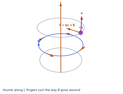
Picture grabbing a wire with your right hand, thumb pointing along the current. Your curled fingers show the field circling the wire. Near the wire the circles are strong; far away they weaken as $1/s$. Bend the wire into a loop, and inside it the circles from every part of the loop all point the same way through the middle, adding to a strong field along the axis.
Another way: steps
Checks. Units: $\mu_0I/\text{length}$ gives tesla. Magnitudes: a $1$ A current makes $20$ μT at $1$ cm from a long wire, less than Earth's field; a $100$-turn coil of radius $5$ cm carrying $1$ A makes $1.3$ mT at its center. Limits: the axial loop field must reduce to $\mu_0I/2R$ at the center and fall as $1/z^3$ far away. And fields must circle currents, never point along or away from them.
Experiments by Biot, Savart and Ampère in 1820, right after Ørsted discovered that currents deflect compasses, showed that the force on a magnet near a wire is perpendicular to both the wire and the line joining them, and falls with distance. The cross product captures that geometry exactly. It also makes the field of a current element zero straight ahead of or behind it, along the line of the current.
The cross product means magnetic fields have a handedness that electric fields lack. Reflect a circuit in a mirror and the current's direction reflects, but the field reverses relative to what a naive reflection would give: $\vec{B}$ is a pseudovector. This subtlety matters in particle physics, where the weak interaction was found in 1957 not to respect mirror symmetry.
The figure shows the field of a long straight wire: rings around it, counterclockwise seen from above for an upward current, as the cross product in the law and the right-hand rule both give.
For a straight segment, measuring angles $\theta$ from the perpendicular to each element, the Biot–Savart integral becomes $\frac{\mu_0I}{4\pi s}\int\cos\theta\,d\theta = \frac{\mu_0I}{4\pi s}(\sin\theta_2 - \sin\theta_1)$. For an infinite wire the angles run from $-90°$ to $90°$, giving $\mu_0I/2\pi s$.
The finite formula lets you build the field of any circuit made of straight pieces. At the center of a square loop of side $a$, each side contributes $\frac{\mu_0I}{4\pi(a/2)}(2\sin 45°)$, and four sides give $2\sqrt{2}\mu_0I/\pi a$, about $10$ percent less than a circular loop whose diameter equals the side. Magnetic field calculations for rectangular coils in motors and sensors use exactly this building block.
Far from a small loop, its field has the same shape as an electric dipole's field: $B_r = \frac{\mu_0}{4\pi}\frac{2m\cos\theta}{r^3}$ and $B_\theta = \frac{\mu_0}{4\pi}\frac{m\sin\theta}{r^3}$, with magnetic moment $m = IA$ pointing along the axis by the right-hand rule. On the axis this matches the large-$z$ limit of the loop formula.
Magnetic dipoles are everywhere. Electrons, protons and nuclei carry intrinsic dipole moments linked to their spin; iron's magnetism comes from aligned electron dipoles; Earth's field is roughly that of a dipole tilted about $10°$ from the rotation axis. Near the surface of Earth the field is $25$ to $65$ μT, and its dipole moment is about $8 \times 10^{22}$ A m² — equivalent to a current of a billion amperes circling the core.
Two coaxial loops separated by their radius produce a field that is remarkably uniform near the midpoint: the second derivative of the field along the axis vanishes there, so the field changes only at fourth order in distance. The center field is $B = (4/5)^{3/2}\mu_0NI/R$.
Physics labs use Helmholtz coils to cancel Earth's field for sensitive measurements, to calibrate magnetometers, and to measure the electron's charge-to-mass ratio in the classic teaching experiment. Larger versions, a few meters across, cancel Earth's field over whole rooms for testing spacecraft magnetometers before launch, as NASA did for missions such as MAVEN and Juno.
A solenoid is many loops stacked along an axis. Adding the axial fields of $n$ turns per unit length over a long solenoid gives $B = \mu_0nI$ inside, independent of position across the interior, and nearly zero outside. At the ends, the field drops to half the interior value, because only one side of the solenoid contributes.
That half-field at the ends is visible in MRI scanners, whose superconducting solenoids produce uniform fields in the central bore and much weaker, rapidly falling fields near the openings. The next lesson derives the solenoid field in one line from Ampère's law, but the Biot–Savart sum over loops is what shows why the field is uniform inside and what happens at the ends.
Magnetic fields add as vectors, like electric fields. Two parallel wires with currents in the same direction produce opposite fields between them, which cancel at the midpoint if the currents are equal; with opposite currents the fields add between the wires and largely cancel far away. Power cords run their two conductors side by side with opposite currents for exactly this reason: their external field falls as $1/s^2$ rather than $1/s$.
Twisting the pair improves the cancellation further, because any residual field from one twist is reversed in the next. Twisted-pair cables in Ethernet networks and telephone lines use this to keep their signals from radiating and to reject interference picked up from outside fields.
Most everyday magnetic fields are small compared with Earth's $50$ μT. A hair dryer produces tens of microtesla a few centimeters away; household wiring, a fraction of a microtesla at a meter. Near a power transmission line carrying $1000$ A, the field $20$ m away is about $10$ μT by the long-wire formula.
Stronger fields appear close to motors and transformers, and the strongest routinely encountered are in MRI machines, $1.5$ to $3$ T, sixty thousand times Earth's field. The National High Magnetic Field Laboratory in Tallahassee, Florida, holds records for continuous fields above $45$ T, produced by stacked resistive and superconducting coils carrying tens of thousands of amperes.
Many experiments need a region with essentially no magnetic field: measuring the neutron's electric dipole moment, testing spacecraft magnetometers, and operating some quantum sensors. Earth's field, $25$ to $65$ μT depending on location, is far too large. Physicists build Helmholtz coils, or sets of three perpendicular pairs, sized to produce an equal and opposite field at the center.
With coils of radius $0.5$ m and $20$ turns, about $1.4$ A cancels $50$ μT. NASA's Goddard Space Flight Center and the Jet Propulsion Laboratory use room-sized coil systems to null Earth's field when calibrating the magnetometers flown on missions to Mars, Jupiter and the Sun. Combined with layers of high-permeability shielding, such systems reach residual fields below a nanotesla, fifty thousand times weaker than Earth's.
A transmission line carrying $1000$ A produces, by the long-wire formula, $10$ μT at $20$ m and $4$ μT at $50$ m — a fraction of Earth's static field, but oscillating at $60$ Hz. Because the three phases of an AC line carry currents that sum to nearly zero, their fields partly cancel, and the actual field falls off faster than a single wire's, roughly as $1/s^2$.
Utilities design line geometry with Biot–Savart calculations to limit fields at the edge of rights-of-way, and arrange phases to maximize cancellation. Decades of research, reviewed by the National Institute of Environmental Health Sciences, have not established that such fields harm health, but the calculations remain standard practice, and the same superposition principle explains why the fields near household wiring are so small.
An electric field points away from a charge, so it is natural to picture a magnetic field pointing along a current. The cross product in the Biot–Savart law says otherwise: each element's field is perpendicular to the element and to the line to the field point, so the field lines are circles around the current. Directly ahead of or behind a current element, its field is zero.
A second error is to treat $\mu_0I/2\pi s$ as the field of any wire. It holds only for a long straight wire, when the field point is close compared with the wire's length. Near the end of a finite wire the field is half as large, and for loops and coils the geometry changes the answer completely.
Consider an element of a loop of radius $R$.
$d\vec{l} \perp \hat{\mathscr{r}}, \qquad \mathscr{r} = R$
Every element is at the same distance and angle.
Write its contribution.
$dB = \dfrac{\mu_0}{4\pi}\dfrac{I\,dl}{R^2}$
All contributions point along the axis.
Integrate around the loop.
$B = \dfrac{\mu_0I}{4\pi R^2} \times 2\pi R$
The total length is the circumference.
Simplify the field.
$B = \dfrac{\mu_0I}{2R}$
Halving $R$ doubles $B$.
Evaluate for $I = 2.0$ A and $R = 5.0$ cm.
$B = \dfrac{4\pi \times 10^{-7} \times 2.0}{2 \times 0.050} = 25\ \mu\text{T}$
Half of Earth's field.
Take a square loop of side $a$ and one side at distance $a/2$ from the center.
$s = \dfrac{a}{2}, \qquad \theta_1 = -45°, \ \theta_2 = 45°$
The side subtends $\pm 45°$ from the center.
Apply the finite-segment formula.
$B_1 = \dfrac{\mu_0I}{4\pi(a/2)}(\sin 45° + \sin 45°) = \dfrac{\mu_0I\sqrt{2}}{2\pi a}$
One side's contribution.
Add the four sides.
$B = 4B_1 = \dfrac{2\sqrt{2}\mu_0I}{\pi a}$
All four point the same way at the center.
Compare with a circle of diameter $a$.
$B_{\text{circle}} = \dfrac{\mu_0I}{a}$
Radius $a/2$.
Form the ratio.
$\dfrac{B_{\text{square}}}{B_{\text{circle}}} = \dfrac{2\sqrt{2}}{\pi} = 0.90$
The circle inscribed in the square gives the larger field.
Interpret the result.
$\text{corners are farther from the center}$
The square's extra wire lies farther away and contributes less.
Two coils of radius $R$, $N$ turns each, are separated by $R$. Write one coil's field at the midpoint.
$B_1 = \dfrac{\mu_0NIR^2}{2(R^2 + R^2/4)^{3/2}}$
The axial formula at $z = R/2$.
Simplify the denominator.
$(R^2 + R^2/4)^{3/2} = \left(\tfrac{5}{4}\right)^{3/2}R^3$
Factor out $R^2$.
Find one coil's field.
$B_1 = \dfrac{\mu_0NI}{2R}\left(\tfrac{4}{5}\right)^{3/2}$
Collect terms.
Add both coils.
$B = \left(\tfrac{4}{5}\right)^{3/2}\dfrac{\mu_0NI}{R} = 0.7155\dfrac{\mu_0NI}{R}$
Both contribute equally at the midpoint.
Evaluate for $R = 0.50$ m, $N = 20$, $I = 1.0$ A.
$B = 0.7155 \times \dfrac{4\pi \times 10^{-7} \times 20 \times 1.0}{0.50} = 36\ \mu\text{T}$
Comparable to Earth's field.
Find the current to cancel $50$ μT.
$I = \dfrac{50}{36} \times 1.0 = 1.39\ \text{A}$
Scale linearly.
Note the uniformity.
$\dfrac{d^2B}{dz^2}\Big|_{\text{mid}} = 0$
The separation $R$ is chosen to make this vanish.
Estimate the uniform region.
$\text{within about } R/5 \text{ of the center, } B \text{ varies by under } 0.1\%$
Enough for most magnetometer calibrations.
Write the long-wire field.
$B = \dfrac{\mu_0I}{2\pi s}$
From integrating Biot–Savart.
Substitute the values.
$B = \dfrac{2 \times 10^{-7} \times 10}{0.05}$
$\mu_0/2\pi = 2 \times 10^{-7}$ T m/A.
Evaluate the field.
A circular loop produces $10$ μT at its center. The same current flows in a loop of twice the radius. What is the field at its center?
Complete the worked solution: two long parallel wires $4$ cm apart carry $9$ A and $6$ A in opposite directions. Find each wire's field at the midpoint and the total, in μT.
Find the first wire's field.
$B_1 = \dfrac{20 \times 9}{2} =$ p
$\mu_0I/2\pi s$ at $2$ cm.
Find the second wire's field.
$B_2 = \dfrac{20 \times 6}{2} =$ q
The same distance.
Add the two fields.
$B = B_1 + B_2 =$ r
Opposite currents circle in opposite senses, so between the wires their fields align.
Match each current to the magnitude of its magnetic field.
| $\mu_0I/2\pi s$ | $\mu_0I/2R$ | $\mu_0IR^2/2(z^2 + R^2)^{3/2}$ | $\frac{\mu_0I}{4\pi s}(\sin\theta_2 - \sin\theta_1)$ | |
|---|---|---|---|---|
| a long wire | ||||
| a loop's center | ||||
| a loop's axis | ||||
| a finite segment |
A loop's field at its center is $744$ μT. Fill in the field on its axis at $z = 0$, $\tfrac{3}{4}R$ and $\tfrac{4}{3}R$, in μT.
| $B$ (μT) | |
|---|---|
| $z = 0$ | |
| $z = \tfrac{3}{4}R$ | |
| $z = \tfrac{4}{3}R$ |
A long straight wire carries $36$ A. What is the magnetic field $2$ cm from it, in μT? Use $\mu_0 = 4\pi \times 10^{-7}$ T m/A.
Answer: μT
A circular loop of radius $12$ cm carries $5$ A. What is the magnetic field on its axis $5$ cm from its center, in μT? Use $\mu_0 = 4\pi \times 10^{-7}$ T m/A.
Answer: μT
To cancel Earth's field of $50$ μT over a sensitive experiment, a lab builds a Helmholtz pair: two coaxial coils of radius $1$ m, $1$ m apart, each with $50$ turns. What current is needed, in amperes?
Answer: A
Lesson test: one question per skill, one attempt each, no hints. Your answers are checked when you submit.
A loop's field at its center is $641$ μT. Fill in the field on its axis at $z = 0$, $\tfrac{3}{4}R$ and $\tfrac{4}{3}R$, in μT.
| $B$ (μT) | |
|---|---|
| $z = 0$ | |
| $z = \tfrac{3}{4}R$ | |
| $z = \tfrac{4}{3}R$ |
You can compute fields from currents. Explain to someone why the field of a wire circles it instead of pointing along it.
19. Your turn: what is the field $5$ cm from a long wire carrying $10$ A?, step 3
$B = 40\ \mu\text{T}$
About Earth's field: enough to deflect a compass.