Back to the on-screen lesson ·
$\vec{E} = -\nabla V$ and $V = k\int dq/\mathscr{r}$: potentials of rings, disks and balls, fields from gradients, Poisson's equation, and the work to move and assemble charges.
Paper packet. Every task here also exists on screen, where it is checked automatically; answers written on paper are not assessed by Nydus. When you are back at a device, enter your answers there.
By the end of this lesson you will be able to compute electric potentials of charge distributions, recover fields by taking gradients, and find the work done moving charges through potential differences.
You know that electrostatic fields have zero curl, Gauss's law in both forms, and potential and potential energy from Physics C. You can take gradients and do integrals in several coordinate systems. This lesson makes the potential the main tool of electrostatics, because a scalar is easier to find than a vector.
| Term | What it means |
|---|---|
| Electric potential | $V(\vec{r}) = -\int_{\mathcal{O}}^{\vec{r}}\vec{E} \cdot d\vec{l}$, the work per unit charge from a reference point. |
| Reference point | Where $V = 0$ is chosen; usually infinity for bounded charges. |
| Gradient | $\nabla V$, the vector of partial derivatives, pointing uphill in $V$. |
| Equipotential | A surface of constant $V$; the field is perpendicular to it. |
| Poisson's equation | $\nabla^2V = -\rho/\varepsilon_0$. |
| Laplace's equation | $\nabla^2V = 0$, which holds wherever there is no charge. |
| Electron volt | The energy an electron gains through $1$ V: $1.602 \times 10^{-19}$ J. |
Since $\nabla \times \vec{E} = 0$, the line integral of $\vec{E}$ between two points does not depend on the path, so we can define
$$V(\vec{r}) = -\int_{\mathcal{O}}^{\vec{r}}\vec{E} \cdot d\vec{l}, \qquad \vec{E} = -\nabla V.$$
One scalar function encodes all three components of the field. For a point charge, with $V = 0$ at infinity, $V = kq/r$, and by superposition any distribution has
$$V(\vec{r}) = \frac{1}{4\pi\varepsilon_0}\int\frac{dq}{\mathscr{r}},$$
a scalar integral with no components to track and a gentler $1/\mathscr{r}$ instead of $1/\mathscr{r}^2$. On the axis of a ring, $V = kQ/\sqrt{z^2 + R^2}$; differentiating, $E_z = -\partial V/\partial z = kQz/(z^2 + R^2)^{3/2}$, the result of lesson 1 with less work.
Putting $\vec{E} = -\nabla V$ into Gauss's law gives Poisson's equation,
$$\nabla^2V = -\frac{\rho}{\varepsilon_0},$$
and in charge-free regions Laplace's equation, $\nabla^2V = 0$. The potential difference between two points is the work per unit charge to move a charge between them: $W = q\,\Delta V$.
Another way: picture
Picture the potential as a landscape of hills and valleys, with positive charges as peaks and negative charges as pits. The field at each point is the direction of steepest descent, scaled by the steepness. A positive charge rolls downhill; a negative charge rolls uphill. Equipotentials are contour lines, and field lines cross them at right angles, just as streams cross contour lines on a map.
Another way: steps
Checks. $V$ must be continuous everywhere, even across surface charges, because the field is finite. Far from bounded charges, $V \to kQ/r$. The field you get by differentiating must match one found another way. And don't use $V = 0$ at infinity for an infinite line or plane: their potentials diverge there, so choose a finite reference point instead.
Computing a field directly means three integrals, one per component, each with its own projection factor. The potential needs one integral with no projections. Symmetry still helps, but even without it the potential integral is simpler because $1/\mathscr{r}$ is gentler than $\hat{\mathscr{r}}/\mathscr{r}^2$. Once you have $V$ everywhere, the field comes from differentiation, which is always easier than integration.
There is a caution. To differentiate, you need $V$ as a function of position near the point, not only its value at the point. The ring's potential on its axis gives the axial field by differentiating with respect to $z$, but it cannot give the sideways field, which requires knowing how $V$ changes off the axis. Know which derivatives your formula can supply.
Outside a uniform ball, $V = kQ/r$. Inside, the field is $kQr/R^3$, and integrating inward from the surface gives $V(r) = \frac{kQ}{2R}\left(3 - \frac{r^2}{R^2}\right)$. At the center, $V = \tfrac{3}{2}kQ/R$, the highest value, even though the field there is zero.
This is the clearest example that field and potential are different things. The field is zero at the center because the potential is at a maximum there — flat on top — not because the potential is zero. Conversely, the potential of a dipole is zero everywhere on the plane midway between its charges, yet the field there is not zero. The field responds to the slope of the potential; the value of the potential depends on the arbitrary choice of reference.
Poisson's equation, $\nabla^2V = -\rho/\varepsilon_0$, packs both laws of electrostatics — zero curl and Gauss's law — into one second-order equation for one unknown. Given the charges and the boundary conditions, it has a unique solution, a fact proved in the next lessons that makes clever guessing a legitimate method.
In empty regions it becomes Laplace's equation, whose solutions have a remarkable property: the value at any point equals the average over any sphere centered there. So a solution of Laplace's equation can have no local maxima or minima inside the region; all its extremes are on the boundary. This is Earnshaw's theorem in disguise: no arrangement of static charges can trap a charged particle in stable equilibrium, which is why ion traps need oscillating fields or magnetic fields.
A charge moving through a potential difference $\Delta V$ gains kinetic energy $-q\,\Delta V$. For an electron, charge $-e$, moving from low to high potential, the gain is $e\,|\Delta V|$. This makes the electron volt a natural unit: an electron accelerated through $1$ V gains $1$ eV $= 1.602 \times 10^{-19}$ J. Chemical bonds are a few eV; visible photons $2$ to $3$ eV; the electrons in an old television tube $25$ keV; the Large Hadron Collider's protons $6.8$ TeV.
Because the gain depends only on the potential difference, not on the path or the shape of the field, electron guns can be designed for focusing without affecting the final energy. Every accelerator, from a dental x-ray tube to Fermilab, is specified first by the potential differences its particles cross.
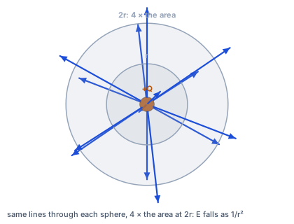
Around the point charge in the figure, the equipotentials are spheres centered on the charge, like the two drawn, and every field line crosses them at right angles.
Since $\vec{E} = -\nabla V$, the field is perpendicular to surfaces of constant potential and points toward lower potential. Where equipotentials crowd together, the field is strong; where they spread apart, it is weak. The surface of a conductor in equilibrium is an equipotential, so field lines leave conductors at right angles.
Mapping equipotentials is how fields were measured before computers: a sheet of resistive paper with electrodes painted on it, and a voltmeter probe tracing lines of equal voltage. Today the same idea appears in medicine. An electrocardiogram measures potential differences across the body produced by the heart's electrical activity; the pattern of equipotentials on the chest, changing through each heartbeat, reveals damage to heart muscle.
Setting $V = 0$ at infinity works only when the charge is confined to a finite region. For an infinite line charge, integrating $2k\lambda/s$ from infinity diverges logarithmically; for an infinite plane, the field is constant and the potential grows linearly without bound. These are artifacts of infinite idealizations: real wires and plates are finite.
The fix is to choose a finite reference. For a line charge, measure from a chosen radius $a$: $V(s) = -2k\lambda\ln(s/a)$. For a coaxial cable, with the outer conductor as reference, the potential difference between the conductors is finite and gives the cable's capacitance per unit length, $2\pi\varepsilon_0/\ln(b/a)$, the number that sets how fast signals travel along it.
The potential is a property of a place: the work per unit charge that the field would do bringing a test charge there from the reference point. Potential energy is a property of a charge at that place, the potential times the charge. A proton and an electron at the same point share a potential but have potential energies of opposite sign, so one is pushed toward lower potential and the other toward higher. Keeping the two ideas separate avoids the most common sign errors in problems about accelerating particles.
The distinction also explains why batteries are rated in volts, not joules. A nine-volt battery raises every coulomb that passes through it by nine joules, whatever the current; how much energy it delivers in total depends on how much charge flows. The same potential difference that sends a trickle of charge through a flashlight bulb can drive a much larger current through a motor, delivering far more energy each second.
The smallest features on research chips and on the masks used to make commercial processors are written with focused electron beams. An electron gun accelerates electrons through tens of kilovolts, typically $50$ or $100$ kV in modern systems, and magnetic lenses focus them to a spot a few nanometers wide that is scanned across a resist-coated wafer.
The accelerating potential sets both the electrons' speed and their wavelength. Through $10$ kV an electron reaches about $5.9 \times 10^7$ m/s nonrelativistically, a fifth of light speed; at $100$ kV relativity matters and the speed is $1.6 \times 10^8$ m/s. Higher voltage means a shorter wavelength and less spreading in the resist, so finer lines. Facilities such as the nanofabrication centers at national laboratories and universities across the United States use these tools to prototype quantum devices and photonic circuits.
Each heartbeat starts with a wave of electrical depolarization spreading through the heart muscle, which acts as a changing electric dipole. The body's tissues conduct, and the dipole sets up potential differences across the skin of about a millivolt. An electrocardiogram measures those differences between electrodes placed on the chest and limbs.
Because the potential of a dipole depends on the direction from the dipole to the electrode, leads at different positions record different waveforms, and together they reveal the direction the heart's dipole points at each moment. Cardiologists read changes in those waveforms to diagnose heart attacks, rhythm disorders and enlarged chambers. Willem Einthoven, who built the first practical instrument, received the 1924 Nobel Prize in Physiology or Medicine; today smartwatches record a single-lead version of the same potential difference.
The field is the slope of the potential, not its height. At the center of a uniformly charged ball the field is zero while the potential is at its highest; on the midplane of a dipole the potential is zero while the field is not. Mixing up the two leads to errors such as concluding that no force acts wherever $V = 0$.
A second error is to treat the value of $V$ as physical. Only potential differences are measurable; adding a constant to $V$ everywhere changes nothing. The choice $V = 0$ at infinity is a convention, convenient for bounded charges and impossible for infinite ones.
Write the potential on the axis.
$V(z) = \dfrac{kQ}{\sqrt{z^2 + R^2}}$
Every piece is the same distance away.
Differentiate with respect to $z$.
$\dfrac{dV}{dz} = kQ \cdot \left(-\tfrac{1}{2}\right)(z^2 + R^2)^{-3/2} \cdot 2z$
The chain rule.
Simplify the derivative.
$\dfrac{dV}{dz} = -\dfrac{kQz}{(z^2 + R^2)^{3/2}}$
Collect factors.
Take the negative gradient.
$E_z = -\dfrac{dV}{dz} = \dfrac{kQz}{(z^2 + R^2)^{3/2}}$
Matches the direct integration of lesson 1.
Note the maximum of $V$.
$V(0) = \dfrac{kQ}{R}, \qquad E(0) = 0$
Flat on top: the field vanishes where the potential peaks.
Write the potential outside.
$V(r) = \dfrac{kQ}{r}, \quad r \ge R$
Like a point charge, with $V = 0$ at infinity.
Write the field inside.
$E(r) = \dfrac{kQr}{R^3}$
From Gauss's law.
Integrate inward from the surface.
$V(r) = V(R) - \displaystyle\int_R^r\dfrac{kQr'}{R^3}\,dr' = \dfrac{kQ}{R} - \dfrac{kQ}{2R^3}(r^2 - R^2)$
$V(b) - V(a) = -\int_a^b E\,dr$.
Simplify the result.
$V(r) = \dfrac{kQ}{2R}\left(3 - \dfrac{r^2}{R^2}\right)$
A downward parabola.
Evaluate at the center.
$V(0) = \dfrac{3kQ}{2R}$
Fifty percent higher than at the surface.
Check Poisson's equation.
$\nabla^2V = \dfrac{1}{r^2}\dfrac{d}{dr}\left(r^2\dfrac{dV}{dr}\right) = -\dfrac{3kQ}{R^3} = -\dfrac{\rho}{\varepsilon_0}$
With $\rho = 3Q/4\pi R^3$.
Bring the first charge $q_1 = 3$ nC in from infinity.
$W_1 = 0$
No other charges are present yet.
Bring $q_2 = -2$ nC to a point $0.10$ m away.
$W_2 = q_2V_1 = q_2\dfrac{kq_1}{0.10}$
Against the potential of the first charge.
Evaluate the second step.
$W_2 = -2 \times 10^{-9} \times \dfrac{8.99 \times 10^9 \times 3 \times 10^{-9}}{0.10} = -5.39 \times 10^{-7}\ \text{J}$
Negative: opposite charges attract.
Bring $q_3 = 1$ nC to a point $0.10$ m from both.
$W_3 = q_3\left(\dfrac{kq_1}{0.10} + \dfrac{kq_2}{0.10}\right)$
The potential of both earlier charges.
Evaluate the third step.
$W_3 = 10^{-9} \times \dfrac{8.99 \times 10^9 \times 10^{-9}}{0.10}(3 - 2) = 8.99 \times 10^{-8}\ \text{J}$
Positive: net repulsion.
Add the steps.
$W = 0 - 5.39 \times 10^{-7} + 0.90 \times 10^{-7} = -4.49 \times 10^{-7}\ \text{J}$
The energy stored in the configuration.
Check with the pair formula.
$W = \dfrac{k}{0.10}(q_1q_2 + q_1q_3 + q_2q_3)$
Summing over pairs; with charges in nC, $k/0.10$ is $8.99 \times 10^{-8}$ J per nC².
Evaluate the pair sum.
$W = 8.99 \times 10^{-8} \times (-5) = -4.49 \times 10^{-7}\ \text{J}$
The order of assembly does not matter.
Relate energy to potential difference.
$\Delta K = e\,\Delta V$
For a charge of magnitude $e$.
Substitute the energy.
$100\ \text{eV} = e\,\Delta V$
The electron volt is defined this way.
Solve for the potential difference.
In a region the potential is $V = 4x^2$ volts, with $x$ in meters. What is the electric field's $x$ component?
Complete the worked solution: a $3$ nC charge is $1$ m from point P and a $-6$ nC charge is $2$ m from P. Find each charge's potential at P and the total, in volts, with $k = 8.99 \times 10^9$ N m²/C².
Find the first charge's potential.
$V_1 = \dfrac{8.99 \times 3}{1} =$ p
$kq/r$ with $q$ in nC gives volts times $10^{-9} \times 10^{9}$.
Find the second charge's potential.
$V_2 = \dfrac{8.99 \times (-6)}{2} =$ q
Negative charge, negative potential.
Add the two potentials.
$V = V_1 + V_2 =$ r
No vector geometry needed.
Match each statement about the potential to its equation.
| $kq/r$ | $-\nabla V$ | $\nabla^2V = -\rho/\varepsilon_0$ | $\nabla^2V = 0$ | |
|---|---|---|---|---|
| a point charge's potential | ||||
| the field from the potential | ||||
| Poisson's equation | ||||
| Laplace's equation |
A uniformly charged ball of radius $R$ has $kQ/R = 549$ V. Taking $V = 0$ at infinity, fill in the potential, in volts, at $r = 0$, $r = R$ and $r = 2R$.
| $V$ (V) | |
|---|---|
| $r = 0$ | |
| $r = R$ | |
| $r = 2R$ |
A ring of radius $6$ cm carries $9$ nC. What is the potential on its axis $8$ cm from its center, in volts, taking $V = 0$ at infinity? Use $k = 8.99 \times 10^9$ N m²/C².
Answer: V
A disk of radius $3$ cm carries $\sigma = 1$ μC/m². How much work, in μJ, is needed to bring a $1$ nC charge from far away to a point on the axis $4$ cm from the disk? Use $\varepsilon_0 = 8.85 \times 10^{-12}$ C²/(N m²).
Answer: μJ
An electron-beam lithography tool accelerates electrons from rest through a potential difference of $5$ kV. Ignoring relativity, how fast do they leave the gun, in units of $10^7$ m/s? Use $e = 1.602 \times 10^{-19}$ C and $m = 9.109 \times 10^{-31}$ kg.
Answer: × 10⁷ m/s
Lesson test: one question per skill, one attempt each, no hints. Your answers are checked when you submit.
A uniformly charged ball of radius $R$ has $kQ/R = 145$ V. Taking $V = 0$ at infinity, fill in the potential, in volts, at $r = 0$, $r = R$ and $r = 2R$.
| $V$ (V) | |
|---|---|
| $r = 0$ | |
| $r = R$ | |
| $r = 2R$ |
You can use the potential to find fields and energies. Explain to someone why the field is zero at the center of a charged ball even though the potential is highest there.
19. Your turn: through what potential difference must an electron fall to gain $100$ eV?, step 3
$\Delta V = 100\ \text{V}$
The electron moves toward higher potential.