Back to the on-screen lesson ·
Reading position, velocity and acceleration graphs: slopes as rates, areas as totals, and the link to the kinematic equations.
Paper packet. Every task here also exists on screen, where it is checked automatically; answers written on paper are not assessed by Nydus. When you are back at a device, enter your answers there.
By the end of this lesson you will be able to read velocities, accelerations and displacements from motion graphs.
From the last two lessons you know position, velocity and acceleration, and the constant-acceleration equations. From math you know how to find the slope of a line and the areas of rectangles and triangles. This lesson ties them together: motion can be read straight off a graph.
| Term | What it means |
|---|---|
| Position-time graph | Position against time; its slope is the velocity. |
| Velocity-time graph | Velocity against time; its slope is the acceleration, its area the displacement. |
| Acceleration-time graph | Acceleration against time; its area is the change in velocity. |
| Slope | Rise over run: the rate one quantity changes with another. |
| Signed area | Area above the time axis counts positive, below it negative. |
| Tangent | A line touching a curve at one point; its slope is the instantaneous rate. |
Graphs of motion carry the same information as the equations, arranged for the eye:
For constant acceleration the velocity-time graph is a straight line, and its area, a trapezoid, reproduces $\Delta x = v_0t + \tfrac{1}{2}at^2$. Areas below the time axis count as negative displacement.
Another way: picture
Picture a car's trip computer drawing a graph of speed as you drive. Where the line climbs steeply you were accelerating hard; where it is flat you were cruising. The total distance you drove is the area under that line, filled in strip by strip, one second's speed times one second at a time. Where the line dips to zero at a red light, no area is added.
Another way: steps
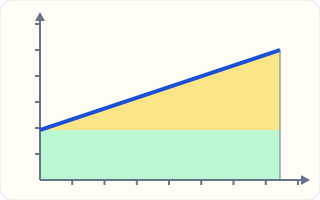
The figure shows a velocity rising steadily from $4$ m/s to $12$ m/s in $8$ s. The area under the line splits into a green rectangle, $8$ s by $4$ m/s, and a yellow triangle, $8$ s by $8$ m/s. The rectangle, $32$ m, is how far the object would go if it kept its starting velocity. The triangle, $32$ m, is the extra gained by speeding up.
Together they give $64$ m, exactly $v_0t + \tfrac{1}{2}at^2$ with $v_0 = 4$ and $a = 1$. The rectangle is the $v_0t$ term; the triangle is the $\tfrac{1}{2}at^2$ term. The equation and the picture say the same thing.
A straight position-time line means constant velocity, and its slope gives the velocity. A curve means changing velocity: the slope at any point, the slope of the tangent line there, is the instantaneous velocity. A curve bending upward means speeding up in the positive direction; bending downward, slowing or speeding up negatively.
Where the curve is flat, at a peak or valley, the velocity is zero: the object is turning around. The height of the graph is the position, not the speed; a very high point simply means far from the origin.
The height of a velocity-time graph is the velocity; above the axis the object moves in the positive direction, below it in the negative. A straight line means constant acceleration, equal to its slope. A horizontal line means constant velocity.
Where the line crosses the time axis, the object stops and reverses. The area above the axis counts as positive displacement and the area below as negative; adding them gives the net displacement, while adding their sizes gives the distance.
For constant acceleration, the acceleration-time graph is a horizontal line. The area under it over a time interval is $a\Delta t$, the change in velocity. A car's crash-test data often comes as an acceleration-time trace, a sharp spike, and the area under the spike gives the car's change in velocity during the collision.
The pattern runs down a ladder: slopes take you from position to velocity to acceleration, and areas take you back up. Calculus makes this exact with derivatives and integrals, as Physics C develops.
Checking an answer. Slopes must have units of the vertical axis over time. Areas must have units of the vertical axis times time. A straight velocity line must give the same displacement as the kinematic equations.
Velocity is the rate position changes, so it appears as the slope of a position graph by definition. Displacement is velocity times time for each small interval; adding up many thin strips of height $v$ and width $\Delta t$ gives the area under the curve.
The same reasoning links acceleration and velocity. For straight-line graphs these are exact geometric facts; for curves they become the derivative and the integral, and the geometric picture still gives the right answer.
Physics labs across the country use ultrasonic motion sensors. The sensor sends a burst of sound many times a second and times its echo from a cart or a person, computing position from the speed of sound. Software then plots position, velocity and acceleration against time as the object moves.
Students walk toward and away from the sensor trying to match a target graph, which quickly teaches that a steeper position line means walking faster and a flat one means standing still. The velocity graph appears noisier than the position graph, because finding slopes magnifies small errors.
Most American cars carry an event data recorder that saves speed, braking and acceleration for a few seconds around a crash. Investigators turn the record into graphs: the slope of the speed graph gives the deceleration, and its area the distance traveled while braking.
The National Highway Traffic Safety Administration sets standards for what these recorders must capture. Combined with skid marks and final positions, the graphs let engineers reconstruct whether a driver braked, how hard, and how fast the car was going at impact.
Words, equations and graphs each suit different questions. An equation gives exact values; a graph shows the whole story at a glance, including when an object stops or turns around; words connect the motion to what actually happens.
Good problem solvers move between them. Sketching a quick velocity-time graph before choosing an equation often reveals the shape of the answer: whether the object reverses, which stage covers the most distance, whether the answer should be positive or negative.
When a velocity graph curves, the area under it can still be estimated by counting grid squares or by splitting it into thin strips. The average velocity over an interval is the area divided by the time, the height of a rectangle with the same area.
Weather services and utilities use the same idea with other quantities: the area under a graph of electric power against time is the energy used, and the area under a graph of river flow against time is the volume of water that passed. Slopes and areas are among the most widely used ideas in science.
A $100$ m sprinter's velocity rises quickly from zero, levels off near a top speed around $10$ to $12$ m/s after $30$ to $60$ m, and may sag slightly near the finish as fatigue sets in. The area under the graph must total $100$ m.
Coaches measure these curves with laser guns and high-speed cameras. A sprinter who reaches a slightly lower top speed but holds it longer can beat one who peaks higher and fades, a comparison that is obvious on the graph but hidden in the final time alone. Splitting the race into ten-meter segments and timing each one turns the graph into a training plan, showing exactly where a runner loses ground.
Before choosing an equation, sketch the velocity-time graph of the motion described. Mark where the object starts, whether the line slopes up or down, and whether it ever crosses the time axis. The sketch takes a few seconds and often reveals the structure of the problem: two stages, a turnaround, a stretch at constant speed.
Physics teachers find that students who sketch first make far fewer sign errors, because the picture shows at once whether a displacement should be positive or negative and whether a speed should be rising or falling. The habit carries on into every later topic, from projectiles to oscillations, where motion graphs remain the clearest way to see what an equation is saying.
High school and college coaches use laser speed guns and timing gates to plot sprinters' velocity against time. A simple model treats the race as steady acceleration to top speed, then constant speed: a velocity graph shaped like a ramp followed by a plateau, with a total area of $100$ m.
For a sprinter reaching $11.5$ m/s after $30$ m, the ramp takes $2 \times 30/11.5 = 5.2$ s and the remaining $70$ m another $6.1$ s, a time of about $11.3$ s. Real sprinters accelerate hardest at the start and keep gaining for $50$ m or more, so the model is only a first sketch, but it shows why the start matters: shortening the ramp by a few meters saves tenths of a second.
When the National Transportation Safety Board investigates a highway crash, one of the first things analysts pull is the vehicle's event data recorder, which logs speed several times a second. The speed-time graph shows whether and when the driver braked: a line sloping down steeply means hard braking.
The slope gives the deceleration, perhaps $7$ m/s² on dry pavement, and the area under the graph before impact gives how far the car traveled while braking. If a car slowed from $30$ m/s to $15$ m/s over $2.1$ s before impact, the area, about $47$ m, and the impact speed of $15$ m/s, about $34$ mph, both come straight from the graph.
It is natural to read a velocity-time graph as a picture of where the object is, so that a line going down means the object moves down or back. A falling velocity line means the object is slowing, if it is above the axis; the object may still be moving forward. Position must be found from the area.
A related error is to find displacement from the slope, or acceleration from the area. Slopes give rates of change; areas give accumulated totals. Checking units tells which is which.
A velocity graph rises from $0$ to $6$ m/s in $3$ s, stays at $6$ m/s for $4$ s, then falls to $0$ in $2$ s. Find the first area.
$\tfrac{1}{2} \times 3 \times 6 = 9\ \text{m}$
Triangle.
Find the middle area.
$4 \times 6 = 24\ \text{m}$
Rectangle.
Find the last area.
$\tfrac{1}{2} \times 2 \times 6 = 6\ \text{m}$
Triangle.
Add the three areas.
$9 + 24 + 6 = 39\ \text{m}$
Total displacement.
Find the average velocity.
$\dfrac{39}{9} = 4.3\ \text{m/s}$
Area over time.
A velocity line runs from $+8$ m/s at $t = 0$ to $-4$ m/s at $t = 6$ s. Find the slope.
$a = \dfrac{-4 - 8}{6} = -2\ \text{m/s}^2$
Constant acceleration.
Find when it crosses zero.
$0 = 8 - 2t \Rightarrow t = 4\ \text{s}$
Turning point.
Find the area above the axis.
$\tfrac{1}{2} \times 4 \times 8 = 16\ \text{m}$
Forward displacement.
Find the area below the axis.
$\tfrac{1}{2} \times 2 \times (-4) = -4\ \text{m}$
Backward displacement.
Find the net displacement.
$16 - 4 = 12\ \text{m}$
Signed sum.
Find the distance traveled.
$16 + 4 = 20\ \text{m}$
Sizes added.
A cart from rest is at $0$, $1.0$, $4.0$ and $9.0$ m at $0$, $1$, $2$ and $3$ s. Test for constant acceleration.
$1, 4, 9 \propto 1^2, 2^2, 3^2$
Distance grows as time squared.
Find the acceleration.
$a = \dfrac{2x}{t^2} = \dfrac{2 \times 1.0}{1^2} = 2.0\ \text{m/s}^2$
From $x = \tfrac{1}{2}at^2$.
Find the velocity at $3$ s.
$v = 2.0 \times 3 = 6.0\ \text{m/s}$
$v = at$.
Find the average velocity over $2$ to $3$ s.
$\dfrac{9.0 - 4.0}{1} = 5.0\ \text{m/s}$
Slope of a chord.
Compare with the instantaneous velocity at $2.5$ s.
$2.0 \times 2.5 = 5.0\ \text{m/s}$
The midpoint, for constant acceleration.
Predict the position at $4$ s.
$\tfrac{1}{2} \times 2.0 \times 16 = 16\ \text{m}$
Continuing the pattern.
Identify the shape.
$\text{a rectangle}$
Constant velocity.
Multiply height by width.
$\Delta x = 5 \times 6$
Area.
Evaluate the displacement.
A velocity-time graph is a straight line from $5$ m/s at $t = 0$ to $15$ m/s at $t = 4$ s. What displacement does it show over that time, in m?
Complete the worked solution: a cart starts from rest at the origin with constant acceleration. A motion sensor records it at $22.5$ m after $3.0$ s and at $90$ m after $6.0$ s. Find its acceleration in m/s², its velocity at $6.0$ s in m/s, and its position at $9.0$ s in m.
Find the acceleration from the first reading.
$a = \dfrac{2x}{t^2} =$ a
From $x = \tfrac{1}{2}at^2$.
Find the velocity at the second reading.
$v = at =$ v
Starting from rest.
Predict the position at the later time.
$x = \tfrac{1}{2}at^2 =$ x
Same rule.
Check the second reading.
$\text{twice the time, four times the distance}$
Distance grows as time squared.
Match each feature of a motion graph to the quantity it gives.
| velocity | acceleration | displacement | change in velocity | |
|---|---|---|---|---|
| slope of a position-time graph | ||||
| slope of a velocity-time graph | ||||
| area under a velocity-time graph | ||||
| area under an acceleration-time graph |
A velocity-time graph rises in a straight line from $0$ to $12$ m/s over $4$ s, then stays flat at $12$ m/s for another $8$ s. Fill in the acceleration during the first stage in m/s², the distance covered in the first stage in m, and the total distance in m.
| value | |
|---|---|
| first-stage acceleration (m/s²) | |
| first-stage distance (m) | |
| total distance (m) |
A straight velocity-time line passes through $(1\ \text{s}, 9\ \text{m/s})$ and $(4\ \text{s}, 3\ \text{m/s})$. Write the velocity, in m/s, as a function of time $t$ in seconds.
Answer:
A cart's velocity rises steadily from $0$ to $12$ m/s in $3$ s, then falls steadily back to $0$ in another $5$ s. How far does it travel, in m?
Answer: m
A high school coach models a sprinter's $100$ m dash: steady acceleration from rest to a top speed of $12.2$ m/s over the first $40$ m, then constant speed to the finish. What time does the model predict, in s?
Answer: s
Lesson test: one question per skill, one attempt each, no hints. Your answers are checked when you submit.
A straight velocity-time line passes through $(1\ \text{s}, 9\ \text{m/s})$ and $(4\ \text{s}, 3\ \text{m/s})$. Write the velocity, in m/s, as a function of time $t$ in seconds.
Answer:
You can read motion graphs. Explain to someone why the area under a velocity-time graph gives displacement.
23. Your turn: a velocity graph is flat at $5$ m/s for $6$ s. What displacement does it show?, step 3
$\Delta x = 30\ \text{m}$
Meters.