Back to the on-screen lesson ·
The wave function as the complete state of a particle, Born's rule $|\Psi|^2dx$ as a probability, normalization, and probabilities of intervals computed exactly.
Paper packet. Every task here also exists on screen, where it is checked automatically; answers written on paper are not assessed by Nydus. When you are back at a device, enter your answers there.
By the end of this lesson you will be able to state what a wave function means, normalize a wave function, compute the probability of finding a particle in an interval, check units and symmetry, and explain why $|\Psi|^2$ is a density and not a probability.
From modern physics you know that particles have wave properties, that the de Broglie wavelength is $h/p$, and that measurement outcomes in quantum physics are probabilistic. From calculus and probability you know how to integrate a polynomial and that a probability density must be integrated to give a probability. This lesson sets out precisely what a wave function is and how every prediction is drawn from it.
| Term | What it means |
|---|---|
| Wave function | $\Psi(x, t)$, a complex-valued function that is the complete description of a particle's state. |
| Born rule | The probability of finding the particle between $x$ and $x + dx$ is $\vert \Psi(x, t)\vert ^2dx$. |
| Probability density | $\vert \Psi\vert ^2$, probability per unit length; only its integral is a probability. |
| Normalization | Scaling $\Psi$ so that $\int\vert \Psi\vert ^2dx = 1$: the particle is certainly somewhere. |
| Normalization constant | The factor $A$ fixed by normalization. |
| Complex conjugate | $\Psi^$, with $i$ replaced by $-i$; $\vert \Psi\vert ^2 = \Psi^\Psi$. |
| Schrödinger equation | $i\hbar\,\partial\Psi/\partial t = -\frac{\hbar^2}{2m}\partial^2\Psi/\partial x^2 + V\Psi$, which governs how $\Psi$ evolves. |
In classical mechanics a particle's state at an instant is its position and momentum. In quantum mechanics it is a wave function $\Psi(x, t)$, a complex-valued function spread over all of space, which evolves according to the Schrödinger equation:
$$i\hbar\frac{\partial\Psi}{\partial t} = -\frac{\hbar^2}{2m}\frac{\partial^2\Psi}{\partial x^2} + V(x)\Psi.$$
Given $\Psi$ at one time, the equation fixes it at all later times — as deterministic as Newton's laws. What is not deterministic is what a measurement finds. Max Born's interpretation, now called the Born rule, gives the link:
$$P(x \text{ to } x + dx) = |\Psi(x, t)|^2dx, \qquad |\Psi|^2 = \Psi^*\Psi.$$
$|\Psi|^2$ is a probability density, probability per unit length. The probability of finding the particle between $a$ and $b$ is its integral, $\int_a^b|\Psi|^2dx$, and because the particle must be somewhere,
$$\int_{-\infty}^{\infty}|\Psi|^2dx = 1.$$
A wave function obeying this is normalized. The Schrödinger equation is linear, so if $\Psi$ solves it so does $A\Psi$ for any constant $A$; normalization is how $A$ is fixed. The equation also preserves normalization over time, which is essential: a probability that drifted away from one would make no sense.
In one dimension, $|\Psi|^2dx$ must be a pure number, so $|\Psi|^2$ has units of inverse length and $\Psi$ itself units of length$^{-1/2}$ — an unusual quantity, and a useful check on any calculation.
Another way: picture
Picture a very large number of identical particles, each prepared in the same state, and each measured once for its position. The results pile up into a histogram. The wave function predicts the shape of that histogram before any measurement is made: $|\Psi|^2$ is its outline, taller where more particles are found. No single particle is spread across the histogram; each lands in one bin.
Another way: steps
Checks. Every probability lies between $0$ and $1$. The probabilities of regions that cover all space add to one. Symmetric densities give symmetric answers — half the probability on each side of the center. The units of $|\psi|^2$ are inverse length, so a normalization constant squared for a polynomial like $x(a - x)$ must carry units of length$^{-5}$. And a wave function that is large where the potential forbids the particle, or that cannot be normalized at all, signals an error upstream.
The function $\psi(x) = Ax(a - x)$ for $0 < x < a$, zero elsewhere, is a smooth approximation to the ground state of a particle in a box: zero at the walls, largest in the middle. Its normalization is
$$\int_0^a A^2x^2(a - x)^2dx = A^2\int_0^a(a^2x^2 - 2ax^3 + x^4)dx = A^2\left(\frac{a^5}{3} - \frac{a^5}{2} + \frac{a^5}{5}\right) = \frac{A^2a^5}{30}.$$
Setting this to one gives $A = \sqrt{30/a^5}$. The probability of finding the particle between $0$ and $ua$ then works out, with the substitution $x = ua$, to
$$P(u) = 10u^3 - 15u^4 + 6u^5.$$
At $u = \tfrac{1}{2}$ this is exactly $\tfrac{1}{2}$, as symmetry demands. At $u = \tfrac{1}{4}$ it is $53/512 \approx 0.104$, far below the $0.25$ a uniformly spread particle would give: the state crowds the particle toward the center and away from the walls. That kind of comparison, between the quantum density and a classical guess, is how to read a wave function.
The wave function is complex because the Schrödinger equation has an $i$ in it. A free particle of momentum $p$ has $\Psi = Ae^{i(px - Et)/\hbar}$, whose real and imaginary parts are cosine and sine waves moving together. Its density, $|\Psi|^2 = |A|^2$, is uniform: a particle of definite momentum is equally likely to be anywhere, which is the uncertainty principle at its most extreme.
The phase of $\Psi$ is not observable by itself — multiplying the whole wave function by $e^{i\alpha}$ changes nothing measurable — but differences in phase between parts of a wave function are. When two parts overlap, their phases decide whether they add or cancel, and that interference is how a single electron, sent through two slits, builds up fringes on a screen one dot at a time.
Born's rule is a statement about the outcomes of measurements. It does not say the particle is smeared out, like a cloud of charge, before it is measured: every position measurement on an electron finds a whole electron, with its whole charge, at one place. Nor does it say the particle was secretly at that place all along — experiments testing Bell's inequalities, met at the end of this course, rule out the simplest versions of that idea.
What happens to the wave function when a measurement is made is the long-running measurement problem, and physicists still disagree about how to describe it. The working rule, which every experiment so far confirms, is simple: compute $|\Psi|^2$, integrate over the region of interest, and that is the fraction of identically prepared systems in which the particle will be found there.
Not every function can describe a particle. A wave function must be normalizable: $\int|\psi|^2dx$ must be finite, so that dividing by it gives total probability one. A constant stretching over all space fails, and so does $1/x$ near the origin. It must also be single-valued, since a probability density has one value at each point, and continuous, because the Schrödinger equation involves its second derivative. Where the potential is finite, its first derivative must be continuous too; only at an infinite wall may the slope jump.
These conditions are not formalities. They are what turns the Schrödinger equation, which has solutions for every energy, into a source of quantized energies: only special energies give solutions that behave well at the walls or die away at infinity. The next unit uses exactly that fact to find the allowed energies of a particle in a box and of a harmonic oscillator.
In 1989 Akira Tonomura's group at Hitachi sent electrons through an electron biprism — the electron version of a double slit — so slowly that only one was in the apparatus at a time, and recorded where each landed on a detector. The first few hundred dots looked random. After ten thousand, the dots had built up bright and dark fringes; after seventy thousand, a clear interference pattern.
Each dot is one whole electron found at one place, exactly as the Born rule says a single measurement must be. The pattern is $|\Psi|^2$, emerging only in the statistics. The wave function behind it is the sum of two parts, one from each path, and where their phases differ by half a cycle the density vanishes: no electron ever lands at those points, although each path alone would put electrons there.
The experiment is often called the most beautiful in physics, because it shows the two halves of the interpretation in one image: definite, particle-like outcomes, and a wave-like probability density that only the accumulated record reveals. Electron microscopes and electron holography, used to image materials atom by atom, rely on exactly the same interference.
The scanning tunneling microscope, invented at IBM in 1981, images surfaces atom by atom by holding a sharp metal tip a few tenths of a nanometer above them. Electrons in the surface have wave functions that leak out into the vacuum, falling off roughly as $e^{-\kappa x}$ with $\kappa \approx 10$ nm⁻¹ for a typical metal.
The current that flows to the tip is proportional to the probability density at the tip, $|\psi|^2 \propto e^{-2\kappa x}$. Moving the tip $0.1$ nm farther away multiplies the current by $e^{-2 \times 10 \times 0.1} = e^{-2} = 0.135$: a single atomic step of about $0.1$ nm changes the current sevenfold. That extreme sensitivity, a direct measurement of the exponential tail of $|\psi|^2$, is what lets the microscope resolve individual atoms.
Binnig and Rohrer received the 1986 Nobel Prize for it, and the technique now also moves single atoms to build structures, such as IBM's "quantum corral" of 48 iron atoms whose interior shows the standing-wave density of the electrons trapped inside.
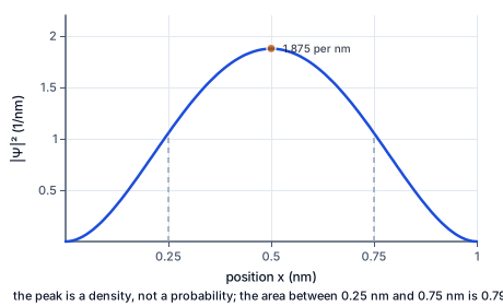
Two errors come from reading $|\Psi|^2$ too literally. The first treats its value at a point as a probability. It is a density, with units of inverse length; the probability of finding a particle at any exact point is zero, and only the integral over an interval gives a probability. A density of $2$ nm⁻¹ is perfectly legal, though a probability of $2$ is not.
The second pictures the particle as physically spread out, its charge or mass distributed like a fog shaped like $|\Psi|^2$. Every measurement contradicts this: a detector registers a whole electron, never a fraction of one, at one place. The shape of $|\Psi|^2$ appears only in the statistics of many measurements on identically prepared particles. Keeping the two levels apart — definite outcomes, probabilistic predictions — is the first discipline quantum mechanics asks for.
A particle has $\psi(x) = Ae^{-|x|/a}$. Write the normalization condition.
$\int_{-\infty}^{\infty}A^2e^{-2|x|/a}dx = 1$
The total probability must be one.
Use the symmetry of the integrand.
$2A^2\int_0^{\infty}e^{-2x/a}dx = 1$
The integrand is even, so integrate over positive $x$ and double.
Evaluate the integral.
$\int_0^{\infty}e^{-2x/a}dx = \dfrac{a}{2}$
The antiderivative is $-\tfrac{a}{2}e^{-2x/a}$, which vanishes at infinity.
Solve for the constant.
$2A^2 \cdot \dfrac{a}{2} = A^2a = 1 \quad\Rightarrow\quad A = \dfrac{1}{\sqrt{a}}$
Only the magnitude of $A$ is fixed; any phase would be unobservable.
Check the units.
$[A] = \text{length}^{-1/2}$
As a one-dimensional wave function must.
A particle has $\psi(x) = Ax(a - x)$ for $0 < x < a$ and zero elsewhere. Write the normalization condition.
$A^2\int_0^a x^2(a - x)^2dx = 1$
The wave function is zero outside the region, so only $0$ to $a$ contributes.
Expand the integrand.
$x^2(a - x)^2 = a^2x^2 - 2ax^3 + x^4$
Square $(a - x)$, then multiply by $x^2$.
Integrate term by term.
$\int_0^a(a^2x^2 - 2ax^3 + x^4)dx = \dfrac{a^5}{3} - \dfrac{a^5}{2} + \dfrac{a^5}{5}$
Each power integrates to $x^{n + 1}/(n + 1)$, evaluated at $a$.
Combine the fractions.
$\dfrac{10 - 15 + 6}{30}a^5 = \dfrac{a^5}{30}$
A common denominator of thirty.
Solve for the constant.
$A^2\dfrac{a^5}{30} = 1 \quad\Rightarrow\quad A = \sqrt{\dfrac{30}{a^5}}$
Positive by convention.
Check the units.
$[A^2] = \text{length}^{-5}, \qquad [A^2x^2(a - x)^2] = \text{length}^{-1}$
The density comes out as inverse length, as it must.
For $\psi = \sqrt{30/a^5}\,x(a - x)$, write the probability of finding the particle between $0$ and $a/4$.
$P = \dfrac{30}{a^5}\int_0^{a/4}x^2(a - x)^2dx$
Born's rule over the interval.
Substitute $x = ua$.
$P = 30\int_0^{1/4}u^2(1 - u)^2du$
$dx = a\,du$, and every power of $a$ cancels.
Expand the integrand.
$u^2(1 - u)^2 = u^2 - 2u^3 + u^4$
The same expansion as before, without $a$.
Integrate and multiply by thirty.
$30\left[\dfrac{u^3}{3} - \dfrac{u^4}{2} + \dfrac{u^5}{5}\right] = 10u^3 - 15u^4 + 6u^5$
A polynomial that runs from $0$ at $u = 0$ to $1$ at $u = 1$.
Substitute $u = \tfrac{1}{4}$ in each term.
$10 \times \dfrac{1}{64} - 15 \times \dfrac{1}{256} + 6 \times \dfrac{1}{1024} = \dfrac{160 - 60 + 6}{1024}$
Over a common denominator of $1024$.
Simplify the expression.
$P = \dfrac{106}{1024} = \dfrac{53}{512} \approx 0.1035$
About one chance in ten.
Compare with a uniformly spread particle.
$P_{\text{uniform}} = \dfrac{1}{4} = 0.25$
The quantum state keeps the particle away from the wall: less than half the classical guess.
Check with the half.
$P\left(u = \tfrac{1}{2}\right) = \dfrac{10}{8} - \dfrac{15}{16} + \dfrac{6}{32} = \dfrac{1}{2}$
Exactly one half, as the symmetry of the density about the center demands.
Write the probability as an integral and use symmetry.
$P = \dfrac{2}{a}\int_0^a e^{-2x/a}dx$
The density is even.
Integrate both sides.
$\dfrac{2}{a}\left[-\dfrac{a}{2}e^{-2x/a}\right]_0^a = 1 - e^{-2}$
The antiderivative evaluated at $a$ and $0$.
Evaluate the result.
An electron's wave function at the point $x = 8$ nm gives $|\psi|^2 = 0.2$ nm⁻¹. What does that number mean?
Complete the worked solution: for $\psi = \sqrt{30/a^5}\,x(a - x)$, find the probability of finding the particle between $0$ and $0.1a$.
Multiply ten by the cube of the fraction.
$10 \times (0.1)^3 =$ a
The first term of the integrated density.
Multiply fifteen by its fourth power.
$15 \times (0.1)^4 =$ b
The second term, subtracted.
Multiply six by its fifth power.
$6 \times (0.1)^5 =$ c
The third term, added.
Combine the three terms.
$P = 10u^3 - 15u^4 + 6u^5 =$ p
The probability of the interval.
For a particle on a line described by $\Psi(x, t)$, with lengths in units of $3$ nm, match each statement to its equation.
| $\int|\Psi|^2dx = 1$ over all space | $\int_a^b|\Psi|^2dx$ | $\text{length}^{-1/2}$ | $\frac{d}{dt}\int|\Psi|^2dx = 0$ | |
|---|---|---|---|---|
| the particle is certainly somewhere | ||||
| the chance of finding it between two points | ||||
| the units of $\Psi$ in one dimension | ||||
| a normalized state stays normalized |
For $\psi = \sqrt{30/a^5}\,x(a - x)$ on $0 < x < a$, the probability of finding the particle between $0$ and $ua$ is $10u^3 - 15u^4 + 6u^5$. For $u = 0.2$, fill in each term and the probability.
| value | |
|---|---|
| $10u^3$ | |
| $15u^4$ | |
| $6u^5$ | |
| probability |
A particle has wave function $\psi(x) = A(a^2 - x^2)$ for $|x| < a$ and zero outside, with $a = 2$ nm. Find $A^2$ in nm⁻⁵ so that $\psi$ is normalized.
Answer: nm⁻⁵
A particle in a region $0 < x < a$ has wave function $\psi(x) = \sqrt{30/a^5}\,x(a - x)$. What is the probability of finding it between $0$ and $0.3a$? Give it to five decimal places.
Answer:
An electron confined along a nanowire of length $a$ has wave function $\psi = \sqrt{30/a^5}\,x(a - x)$. A probe senses only the stretch from three tenths to seven tenths of the way along. What is the probability of finding the electron there? Give it to five decimal places.
Answer:
Lesson test: one question per skill, one attempt each, no hints. Your answers are checked when you submit.
For $\psi = \sqrt{30/a^5}\,x(a - x)$ on $0 < x < a$, the probability of finding the particle between $0$ and $ua$ is $10u^3 - 15u^4 + 6u^5$. For $u = 0.1$, fill in each term and the probability.
| value | |
|---|---|
| $10u^3$ | |
| $15u^4$ | |
| $6u^5$ | |
| probability |
You can normalize a wave function and compute probabilities from it. Explain to someone why a detector always finds a whole electron even though its wave function is spread out.
16. Your turn: for $\psi = e^{-|x|/a}/\sqrt{a}$, what is the probability of finding the particle between $-a$ and $a$?, step 3
$P = 1 - 0.1353 = 0.8647$
Nearly nine chances in ten within one decay length of the center.